Name and Year of Study	Country	Data Period	Study Findings
Durmaz and Jie (2024)	Mexico	2000 - 2022	Study findings supported a long run cointegrating real money demand function. The findings do not support asymmetric effects of the exchange rate on real money demand
Ogbaro et al (2023)	Nigeria	1981 - 2020	Study findings confirmed that financial innovation has asymmetric effects on real money demand. Their findings confirm that financial innovation has asymmetric effects on money demand, with only changes in the financial innovation positive partial sums having significant effects on both the short run and long run. Study findings also confirmed that financial innovation has not led to real money demand instability.
Shu et al (2023)	China	1994q1- 2017q3	The study findings show that both narrow (M1) and broad money (M2) are nonlinearly related to real GDP, interest rate, inflation rate, the effective exchange rate of RMB, and the trade variable.
Siklar et al (2021)	Turkey	1986 - 2020	The study findings support a long run cointegrating relationship between real money demand and the key determinants, real income, the price level and interest rate (opportunity cost).
Kayongo (2020)	Uganda	2008q3– 2018q4	The study findings confirm that the exchange rate has asymmetric effects on real money demand. Uganda Shilling depreciation negatively affects real money demand in Uganda while exchange rate appreciation positively effects real money demand.
Mahmood et al (2018)	Saudi Arabia	1968 - 2018	The study finding supports long run money demand stability and confirm that real income is positively related to money demand while inflation has negative effects on real money demand.

Table 1.1: Selected Nonlinear Autoregressive Distributed Lag models (Country Studies)

Variable	Unit Root Test (In Levels)			Unit Root Test (First Difference)
		t statistic	prob.		t statistic	prob.
Lrmd3zzw	ADF test	-2.000	0.2853	ADF test	-3.1472	0.0025
	Test Critical values 1% level:	-3.6161		Test Critical values 1% level:	-2.6272
	5% level:	-2.9412		5% level:	-1.9498
	10% level:	-2.609		10% level:	-1.6115
LCPI	ADF test	-1.1392	0.9155	ADF test	-2.951	0.0036
	Test Critical values 1% level:	-4.0739		Test Critical values 1% level:	-2.5935
	5% level:	-3.4655		5% level:	-1.9448
	10% level:	-3.1594		10% level:	-1.6142
LGDP	ADF test	-2.4749	0.9091	ADF test	-5.2308	0.001
	Test Critical values 1% level:	-4.9491		Test Critical values 1% level:	-4.9491
	5% level:	-4.4436		5% level:	-4.4436
	10% level:	-4.1936		10% level:	-4.1936
LRMD3FC	ADF test	-1.7873	0.7010	ADF test	-6.6242	0.000
	Test Critical values 1% level:	-4.0868		Test Critical values 1% level:	-2.597
	5% level:	-3.4716		5% level:	-1.9453
	10% level:	-3.1629		10% level:	-1.6138
Zinflr	ADF test	-2.5762	0.0010
	Test Critical values 1% level:	-2.597
	5% level:	-1.9453
	10% level:	-1.6138

Table 2: The table below shows the results of the unit root tests.

Dependent Variable: DLOG(RMD3ZZW)
Method: ARDL
Date: 04/25/26 Time: 13:16
Sample: 2019M03 2023M12
Included observations: 58
Dependent lags: 4 (Automatic)
Automatic-lag linear regressors (3 max. lags): LOG(GDP) LOG(RMD3FC)
Automatic-lag dual non-linear regressors (3 max. lags): ZINFLR
Static regressors: DUM2309 DUM19M9 DUM21M3 DUM22M4
DUM23M7 DUM20M1 DUM23M2
Deterministic: Restricted constant and no trend (Case 2)
Model selection method: Akaike info criterion (AIC)
Number of models evaluated: 256
Selected model: ARDL(2,2,3,2)
Variable	Coefficient	Std. Error	t-Statistic	Prob.*
LOG(RMD3ZZW(-1))	-0.234996	0.043503	-5.401862	0
LOG(GDP(-1))	-1.937357	0.292599	-6.621199	0
LOG(RMD3FC(-1))	0.29022	0.037287	7.78347	0
@CUMDP(ZINFLR(-1))	-0.009338	0.001281	-7.288582	0
@CUMDN(ZINFLR(-1))	-0.005709	0.00126	-4.531579	0.0001
C	9.701935	1.273108	7.62067	0
DLOG(RMD3ZZW(-1))	-0.395972	0.098221	-4.031429	0.0003
DLOG(GDP)	-1.651137	1.962252	-0.84145	0.4058
DLOG(GDP(-1))	-4.909462	1.955418	-2.510697	0.0168
DLOG(RMD3FC)	0.168127	0.038364	4.382442	0.0001
DLOG(RMD3FC(-1))	-0.103854	0.041167	-2.522759	0.0163
DLOG(RMD3FC(-2))	-0.266557	0.053829	-4.951961	0
@DCUMDP(ZINFLR)	-0.010027	0.001033	-9.702367	0
@DCUMDN(ZINFLR)	-0.004052	0.001478	-2.74119	0.0096
@DCUMDP(ZINFLR(-1))	-0.000444	0.001361	-0.326364	0.7461
@DCUMDN(ZINFLR(-1))	0.003317	0.001012	3.278168	0.0024
DUM2309	-0.240218	0.040461	-5.937056	0
DUM19M9	-0.217708	0.039275	-5.54313	0
DUM21M3	-0.095871	0.037877	-2.531108	0.016
DUM22M4	0.162742	0.038159	4.264886	0.0001
DUM23M7	0.177425	0.052627	3.371349	0.0018
DUM2020	-0.10043	0.038644	-2.598835	0.0136
DUM23M2	-0.092833	0.037626	-2.467286	0.0187
R-squared	0.925888	Mean dependent var		0.003513
Adjusted R-squared	0.879303	S.D. dependent var		0.09611
S.E. of regression	0.03339	Akaike info criterion		-3.67311
Sum squared resid	0.039021	Schwarz criterion		-2.856038
Log likelihood	129.5202	Hannan-Quinn criteria.		-3.354844
F-statistic	19.87532	Durbin-Watson stat		1.952467
Prob(F-statistic)	0

Table 1.2: The Local Currency Real Money Demand NARDL Model

Null hypothesis: No levels relationship
Number of cointegrating variables: 4
Trend type: Rest. constant (Case 2)
Sample size: 58
Test Statistic	Value
F-statistic	24.050841

Bounds Test

	0.1		0.05		0.01
Sample Size	I(0)	I(1)	I(0)	I(1)	I(0)	I(1)
55	2.345	3.280	2.763	3.813	3.738	4.947
60	2.323	3.273	2.743	3.792	3.710	4.965
Asymptotic	2.200	3.090	2.560	3.490	3.290	4.370
* I(0) and I(1) are respectively the stationary and non-stationary bounds.

Bounds Critical Values

Coefficient symmetry tests
Null hypothesis: Coefficient is symmetric
Degrees of freedom (simple tests): F(1,35), Chi-square(1)
Degrees of freedom (joint tests): F(2,35), Chi-square(2)
Equation: EQ000101RMD3ZZW
Variable	Statistic	Value	Probability
Long run
ZINFLR	F-statistic	27.10329	0.0000
	Chi-square	27.10329	0.0000
Short run
ZINFLR	F-statistic	10.85659	0.0023
	Chi-square	10.85659	0.0010
Joint (Long-Run and Short-Run)
ZINFLR	F-statistic	15.93556	0.0000
	Chi-square	31.87113	0.0000

Table 6

Months	1	2	3	4	5	6	7	8	9	10	11	12	Cumulative Shocks impact on local currency real money demand
1	1												1.00
2	0.77	1.00											1.77
3	0.59	0.78	1.00										2.37
4	0.45	0.61	0.78	1.00									2.84
5	0.34	0.48	0.61	0.78	1.00								3.21
6	0.26	0.37	0.48	0.61	0.78	1.00							3.51
7	0.20	0.29	0.37	0.48	0.61	0.78	1.00						3.74
8	0.15	0.23	0.29	0.37	0.48	0.61	0.78	1.00					3.92
9	0.12	0.18	0.23	0.29	0.37	0.48	0.61	0.78	1.00				4.06
10	0.09	0.14	0.18	0.23	0.29	0.37	0.48	0.61	0.78	1.00			4.18
11	0.07	0.11	0.14	0.18	0.23	0.29	0.37	0.48	0.61	0.78	1.00		4.26
12	0.05	0.09	0.11	0.14	0.18	0.23	0.29	0.37	0.48	0.61	0.78	1.00	4.33
13	0.04	0.07	0.09	0.11	0.14	0.18	0.23	0.29	0.37	0.48	0.61	0.78	3.39
14	0.03	0.05	0.07	0.09	0.11	0.14	0.18	0.23	0.29	0.37	0.48	0.61	2.65
15	0.02	0.04	0.05	0.07	0.09	0.11	0.14	0.18	0.23	0.29	0.37	0.48	2.07
16	0.02	0.03	0.04	0.05	0.07	0.09	0.11	0.14	0.18	0.23	0.29	0.37	1.62
17	0.01	0.03	0.03	0.04	0.05	0.07	0.09	0.11	0.14	0.18	0.23	0.29	1.27
18	0.01	0.02	0.03	0.03	0.04	0.05	0.07	0.09	0.11	0.14	0.18	0.23	0.99
19	0.01	0.02	0.02	0.03	0.03	0.04	0.05	0.07	0.09	0.11	0.14	0.18	0.77
20		0.01	0.02	0.02	0.03	0.03	0.04	0.05	0.07	0.09	0.11	0.14	0.60
21			0.01	0.02	0.02	0.03	0.03	0.04	0.05	0.07	0.09	0.11	0.46
22				0.01	0.02	0.02	0.03	0.03	0.04	0.05	0.07	0.09	0.35
23					0.01	0.02	0.02	0.03	0.03	0.04	0.05	0.07	0.26
24						0.01	0.02	0.02	0.03	0.03	0.04	0.05	0.20
25							0.01	0.02	0.02	0.03	0.03	0.04	0.14
26								0.01	0.02	0.02	0.03	0.03	0.10
27									0.01	0.02	0.02	0.03	0.07
28										0.01	0.02	0.02	0.05
29											0.01	0.02	0.03
30												0.01	0.01

Table 1.3: Cumulative 1% inflation shocks (12 months) on local currency real money demand

	NARDL Model Parameters	Long Run Coefficient
LOG(RMD3ZZW(-1))	-0.234996
LOG(GDP(-1))	-1.937357	-8.24
LOG(RMD3FC(-1))	0.29022	1.23
@CUMDP(ZINFLR(-1))	-0.009338	-0.04
@CUMDN(ZINFLR(-1))	-0.005709	0.02

Table xxx: Long run NARDL Coefficients

Breusch-Godfrey Serial Correlation LM Test:
Null hypothesis: No serial correlation at up to 2 lags
F-statistic	0.079831	Prob. F(2,33)	0.9235
Obs*R-squared	0.279265	Prob. Chi-Square(2)	0.8697

LM Test for Serial Correlation

Heteroskedasticity Test: Breusch-Pagan-Godfrey
Null hypothesis: Homoskedasticity
F-statistic	1.226858	Prob. F(22,35)	0.2878
Obs*R-squared	25.25325	Prob. Chi-Square(22)	0.2851
Scaled explained SS	6.974911	Prob. Chi-Square(22)	0.999

Heteroscedasticity Test

Test	Method used	p-value	Conclusion
Autocorrelation Test	Breusch-Godfrey Serial Correlation	0.8997	No Autocorrelation
Heteroscedasticity Test	Breusch-Pagan Godfrey Test	0.9990	No Heteroskedasticity
Normality Test	Jarque-Bera Test	0.7069	Error term is normally distributed
Stability Test	Cusum of Squares		Model parameters are stable

Specification and Diagnostic Test Summary

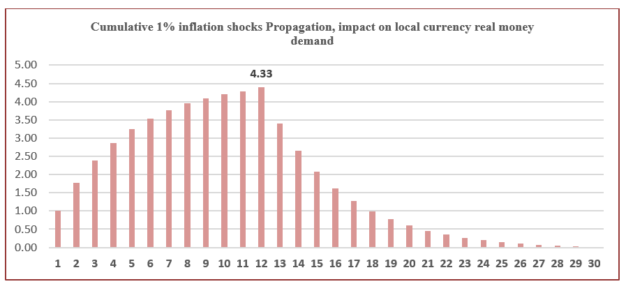Figure 1.1: Cumulative 1% shocks to inflation (12 months), impact on local currency real money demand

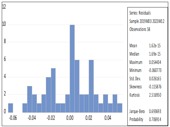Figure 2: Histogram

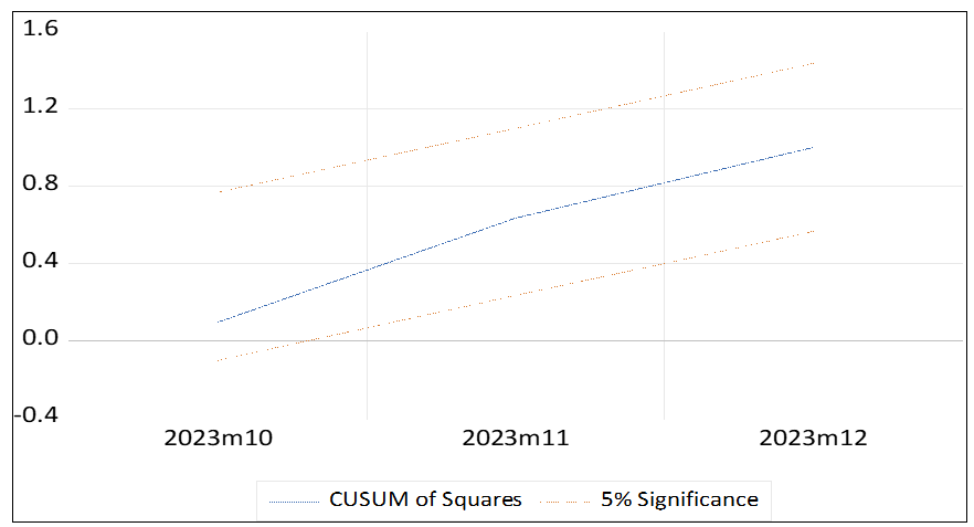Stability Test (Cusum of Squares)

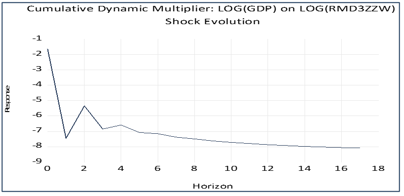Figure 1.8.1: A shock to real GDP, impact on the local currency real money demand

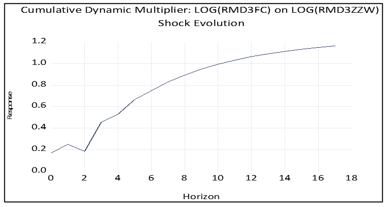1.8.2: A shock to foreign currency real money demand

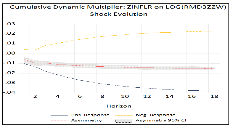1.8.3: Cumulative Positive and Negative shocks to the inflation rate

1.1 Introduction

The paper examines the long run cointegrating relationship between inflation and the local currency real money demand. Further, the paper explores the asymmetric effects of the inflation shocks on the local currency real money demand in Zimbabwe, to investigate the hypothesis of symmetry – whether positive and negative shocks to partial sums of the inflation rate have symmetrical effects on the local currency real money demand. The study applies the nonlinear autoregressive distributed lag (NARDL) model on monthly data for the multicurrency period from 2019:01 – 2023:12.

The model decomposes inflation into positive and negative partial sums, to determine the impact of changes to the partial sums on the local currency real money demand. The null hypothesis is that shocks to the positive and negative partial sums of inflation have symmetrical effects on the local currency real money demand.

The paper is organised as follows: First, a theoretical overview, followed by unit root tests to determine the variables order of integration, and estimation of the NARDL model. The bounds tests for long run cointegration confirmed long run cointegration. Tests for symmetry were undertaken, followed by analysis of the long run and short run dynamics. The model was subjected to specification and diagnostic tests. The short run dynamic impact multipliers characterise how the model adjusts towards equilibrium following a shock.

1.2 Theoretical Overview

Monetary policy formulation is conducted on the basis of a strong assumption that the economy responds symmetrically to a monetary expansion, as to a monetary contraction. In the same analysis, by implication, also the assumption that inflation shocks have symmetrical effects on the local currency real money demand function. In practice, firms and households often respond unevenly to a monetary contraction or expansion and inflation shocks often have asymmetrical effects on economic activity and therefore, the local currency real money demand.

The Nonlinear Autoregressive Distributed Lag (NARDL) model explores the assumption of asymmetric effects of monetary shocks on the exchange rate. The paper follows the seminal work of Shin, Yu, Greenwood and Nimmo (2014), as a further expansion of the autoregressive distributed lag (ARDL) model developed by Pesaran, Shin and Smith (2001).

Pesaran, Shin and Smith proposed modelling cointegration using the ARDL model (2001) in which a variable is regressed on its own lags and lags of the explanatory variables. Within this framework, cointegration and therefore long run relationship could be proven through Bounds testing, to determine the existence of either long run or short run relationship. Through Bounds testing, they generated consistent, unbiased estimators (BLUE) from a combination of stationary and non-stationary variables. Further, through the dynamic multipliers, they were able to characterise the dynamics of adjustment following a shock.

As a progression to Pesaran, Shin and Smith (2001), Shin et al. (2014) expanded on the ARDL framework and suggested a method for modelling asymmetric cointegration and dynamic multipliers in a NARDL framework. They decomposed the explanatory variables into positive and negative partial sums and introduced short run and long run nonlinearities, hence the Nonlinear Autoregressive Distributed Lag model. Through the NARDL model, the idea is to test whether positive and negative shocks have symmetrically distributed effects on the endogenous variable.

Shin et al follow Pesaran et al. (2001) and use a Bounds testing approach to test for the existence of a stable long-run relationship, which is valid irrespective of whether the underlying regressors are I(0), I(1), or mutually cointegrated. The sets of critical values proposed by Pesaran et.al (2001), provide a band covering all three possible classifications - cointegration, no cointegration or indeterminate.

Shin et al. (2014) drew attention to the vast literature developed over the decades around the time series analysis and modelling non-stationary variables, commencing with the seminal work of (Dickey and Fuller 1979; Engle and Granger 1987; Johansen 1988; Kwiatkowski et al. 1992), Phillips and Hansen (1990). These represent major theoretical landmarks in time series modelling.

Shin et al (2014) extended the work and developed a “flexible nonlinear dynamic framework that is capable of simultaneously and coherently modelling asymmetries both in the underlying long-run relationship and in the patterns of short run dynamic adjustment”. They derive a dynamic error correction associated with the asymmetric long run cointegrating regression, hence the nonlinear autoregressive distributed lag (NARDL) model. They also derive asymmetric cumulative dynamic multipliers that permit the simulation of the asymmetric adjustment patterns following positive and negative shocks to the explanatory variables. Following the same approach, there have been several studies that employed a NARDL framework to analyse and model time series variables, as below.

Table 1

1.3 Data Sources and Unit Root tests

The data for the study was collected from various sources, listed below:

• Central Statistical Office (Zim Stats);
• Reserve Bank of Zimbabwe Monthly Economic Review (various)
• IMF Country Data
• Federal Reserve Economic Data (FRED)

The time series data was subjected to extensive analysis to ascertain the nature of the data generating process. The Log transformation was carried on the variables in levels.

Unit Root Tests

Unit root tests were performed on each of the model variables to establish the order of integration. The variables are nonstationary in levels and first difference stationary (the variables are stationary after first differencing, I(1).

Table 2

1.4 Empirical Model

Nonlinear Autoregressive Distributed Lag Model

The study explores inflation shocks asymmetric effects on the local currency real money demand function the Nonlinear Autoregressive Distributed Lag (NARDL) model. The objective is to determine whether positive shocks to inflation and negative shocks to inflation have symmetrically distributed effects on the local currency demand. This has implications for both the timing and magnitude of monetary policy changes.

The asymmetric long-run regression model is given by:

Where:

Y_t is the dependent variable at time t.

β₀ is the intercept term.

Β⁺¹ and B^-1 are the coefficients for the positive (X_t+) and negative (X_t-) changes in the independent variable X, respectively.

µ_t is the error term at time t.

Decomposition of X into X⁺ and X^-

In this model, the independent variable X is decomposed into two parts:

X⁺: Captures the positive changes in (positive partial sums of inflation).

X^-: Captures the negative changes in X (negative partial sums of inflation).

This decomposition allows the model to account for different impacts of positive and negative changes in the independent variable on the dependent variable.

1.5 Nonlinear Autoregressive Distributed Lag Local Currency Real Money Demand

The Nonlinear Autoregressive Distributed Lag model estimation results in the table below:

The NARDL price level equation is estimated using monthly data (2019m1 - 2023M12)

Table 3

Cointegration Bounds Tests

The Bounds Test for Cointegration is suitable particularly for small sample data, and variables have a mixed order of integration (1(0) and I(1), but not I(2). The approach is a joint significance test of the lagged variables.

Table 4

Table 5

H0: No Levels relationship (no long run cointegration)

H1: Levels relationship exists (Cointegration)

The Bounds Test results show that there exists a cointegrating long run relationship between the local currency real money demand and explanatory variables.

Symmetry Test

The test seeks to establish whether the positive and negative shocks to inflation have symmetrically distributed effects on the local currency real money demand. The standard ARDL model assumes linear symmetry, while the Nonlinear (NARDL) model tests for asymmetries, using partial sum decompositions of variables to assess long-run or short-run asymmetries through the Pesaran-Shin-Smith F-bounds.

Table 6

H0: Inflation shocks have symmetrical effects on local currency real money demand

H1: Inflation shocks have asymmetrical effects on local currency real money demand

Table 7

The test results lead to rejection of the null hypothesis and acceptance of the alternative hypothesis that inflation shocks have asymmetrical effects on the local currency real money demand function, for both the short run and the long run.

1.6 Interpretation of Results

Error Correction Term (LOG(CPI(-1)))

The local currency real money demand NARDL equation is a cointegrating model, with an adjustment coefficient of -0.235, implying that as much as 23.5% of the departure from equilibrium is corrected every month. This implies persistence and shows that following any inflation shock to real money demand, the effects of the shock persist in the economy for at least 18 months, as the economy adjusts gradually to a new equilibrium. By extension this also means that where the economy experiences inflation shocks for 12 successive months, the impact on the local currency real money demand persists in the economy for a cumulative total period of 30 months, as shown in the table below:

The figure below shows the cumulative inflation shocks propagation following successive 1% shocks to inflation for twelve (12) months. The maximum impact is 4.33 times larger than the initial single period shock, showing that the local currency real money demand will be 4.33 times lower after 12 months of successive 1% shocks to inflation, ceteris paribus.

Figure 1

Long run determinants

The table below shows the long run coefficients.

Table 8

In the long run, the local currency real money demand function is:

Inversely related to real GDP (a 1% increase to real GDP leads to a decline in local currency demand by 8.24%. This is not consistent with macroeconomic theory and reflects the impact of extensive dollarisation during the Multicurrency ZWL era period since 2019);

Directly related to foreign currency real money demand (a 1% increase in foreign currency real money demand leads to a 1.23% increase in the local currency real money demand;

A 1% positive shock to the cumulative positive partial sums of inflation to a 0.04% decrease in the local currency real money demand in the long run.

A1% negative shock to the cumulative negative partial sums of inflation leads to a 0.02% increase in the local currency real money demand.

Real GDP (LOG(GDP(-1))

The lagged real GDP (scale factor) has a long run coefficient of -8.24 and is statistically significant at 1%. The expectation was for a positive relationship between real GDP and local currency real money demand. In the case for Zimbabwe, during the Multicurrency ZWL era (2019 – 2023), real GDP growth is inversely related to local currency real money demand and explains why the local currency usage has progressively shrunk (local currency share of broad money shrank to 18.5% by December 2025) while the economy has experienced a cumulative real GDP growth of 21.6% (2021 -2024) since the Covid19 pandemic (Zimstats).

Foreign currency real money demand (Log(RMD3FC))

The local currency real money demand is positively related to the foreign currency real money demand. A 1% increase in the foreign currency real money demand leads to a 1.23% increase in demand for local currency real money demand in the long run. This relationship is amplified by contemporaneous short run dynamics but moderated by lagged effects

Asymmetric Effects (CumDP(Zinflr(-1)) and CumDN(Zinflr(-1)))

Shocks to inflation have asymmetric effects on the local currency real money demand function. A 1% increase in the cumulative positive partial sums of inflation lead to a long run 0.04% decline in the local currency real money demand (-0.009338, p<0.01).

A 1% shock to the negative partial sums of inflation (decrease in inflation) leads to a long run 0.02% increase in the local currency real money demand ((-0.0057, p<0.01). The impact of positive partial sums of inflation is double the impact of a decrease in inflation, confirming asymmetry.

The asymmetric effects are compounded in both directions (positive and negative) by short run dynamics. Short run positive shocks to inflation reinforce the decline in local currency real money demand, while short run negative shocks to inflation reinforce the increase in local currency demand. This is consistent with macroeconomic theory and suggests that the local currency real money demand responds to both inflation shocks as well disinflation. However, the pace of local currency real money demand response to disinflation is significantly lower. The sluggish response mainly reflects embedded inflation expectations in the economy, creating inertia.

Short run dynamics

Lagged changes Local Currency Real money demand (DLOG(RMD3ZZW(-))

The lagged first difference of the local currency real money demand function has a negative coefficient of -0.2765, compounding the decline in the local currency real money demand following a shock to inflation, and is statistically significant at 1% ((-0.395, p<0.01). This is consistent with macroeconomic theory, notably for an economy dominated by inflation inertia.

This also indicates that inflationary shocks propagate through the economic system with considerable momentum, reflecting indexation mechanisms and institutionalised inflation expectations following Zimbabwe's hyperinflationary history (Coorey et al., 2007; McIndoe-Calder, 2018). The persistence of price shocks, evident in the three lag structure, confirms that inflation in Zimbabwe exhibits strong inertia and persistence.

Changes in Real GDP (DLOG(GDP))

The lagged real GDP changes (-1.27, p<0.06) compounds the decline in the local currency real money demand , following an increase in real GDP. An increase in real GDP leads to further contraction in the demand for local currency real money demand, reflecting the interplay and dominance of foreign currency balances in driving economic activity (and therefore growth) in Zimbabwe, during the Multicurrency ZWL era (2019 – 2023).

Changes in Foreign currency real money demand (Dlog(RMD3FC)

The changes to foreign currency real money balances have multiple dynamics on the local currency real money demand. The contemporaneous impact (DLOG(RMD3FC) has an immediate positive effect (0.166, p<0.01), significant at 1%; while lagged effects (lag 1 and 2) have moderating effects and also significant at 1%.

Short run dynamics – Changes in Inflation (DCUMDP(Zinflr) and DCUMN(Zinflr)

The short run positive shocks to inflation DCUMDP(Zinflr) reinforce the decline in local currency real money demand (-0.00933, p<0.01). The short run negative shocks to inflation reinforce the increase in local currency demand (-0.00274, p<0.01). The pace of local currency real money demand response to disinflation is significantly lower.

Dummy Variables

The seven dummy variables capture discrete events and policy shifts which affected the economy and the local currency real money demand. The dummy variables are:

Dum19M9; Dum20M1; Dum21M3; Dum22M4; Dum23M2; Dum23M7; Dum23M9 (all statistically significant at 1%).

The dummy variables capture exogeneous shocks (Covid19 pandemic), policy shifts (such as the policy to stop bank credit in April 2022) and the policy to allow the exchange rate to float from May 2023, leading to rapid depreciation of the local currency exchange rate.

1.7: Specification and Diagnostic Tests

The NARDL model Specification and Diagnostic Tests are below:

Figure 2

The JB Test statistic shows that the residuals are normally distributed.

Table 9

The LM Test results show that the residuals have no serial correlation

Table 10

The Heteroscedasticity test results show that the model has no multiple variances.

Figure 3

The Cusum of squares results show that the parameters are stable.

Table 11

The specification and diagnostic tests confirm the statistical adequacy of the estimated NARDL model.

1.8 Dynamic Multipliers

1.8.1 A shock to real GDP, impact on local currency real money demand

Figure 4

The dynamic multiplier traces the cumulative response of the local currency real money demand to a one unit shock to real GDP. The results show that a 1% shock to real GDP immediately triggers a decline in the local currency real money demand by a magnitude of 7.5% in the first month and thereafter gradually declines to about 8% in the long run (15 -18 months). In the unique case of Zimbabwe, real GDP growth is inversely related to the local currency real money demand.

Figure 5

The local currency real money demand is positively related to the local currency real money demand. A 1% shock to the foreign currency real money demand leads to a 0.2% increase after two months, a 0.3% increase after 3 months, a 1% increase after 10 months and a long run value of 1.2% (18 months).

Figure 6

The cumulative positive partial sums and cumulative negative partial sums of the inflation rate have asymmetric effects on the local currency real money demand. A 1% positive shock to the inflation rate instantly and progressively reduces the local currency real money demand, by a magnitude 0.02% after 4 months, 0.03% after 8 months, 0.035% after 12 months and 0.04% in the long run (after 18 months).

A negative shock to the inflation rate increases the local currency real money demand by 0.01% after 4 months, 0.02% after 12 months and 0.022% in the long run (after 18 months).

The Asymmetry 95% Confidence Interval is below 0.00, confirming that positive and negative shocks to inflation have asymmetrically distributed effects on local currency real money demand.

1.9 Conclusion and Monetary Policy Implications

Positive and negative shocks to the inflation rate in Zimbabwe have asymmetrically distributed effects on the local currency real money demand and subject to long lags. The positive shocks to the inflation rate impact on the local currency real money demand is significantly larger than the negative shocks to inflation.

Real GDP is inversely related to the local currency real money demand, while foreign currency real money demand is positively related to the local currency real money demand. This has implications for the de-dollarisation strategy for Zimbabwe. Durable de-dollarisation can only be achieved in the very long run, as the local currency real money demand responds very slowly to disinflation (negative shocks to inflation). However, the process must begin with calibration of credit growth rates to ensure that ZiG credit growth rate is consistently higher than USD credit growth rate overtime while ensuring equilibrium, currency and exchange rate stability.

References

1. Adil MH, et al. (2024) Money demand function in India: Evidence with multiple structural breaks, Indian Economic Review, 59: 78-102.
2. Abubakar A, Lawal AI (2022) Monetary policy transmission mechanism in Sub-Saharan Africa, Journal of African Economies, 31: 145-68.
3. Akinbobola TO (2012) The dynamics of money supply, exchange rate and inflation in Nigeria, Journal of Applied Finance & Banking, 2: 117-41.
4. Allen DE, McAleer M (2020) A Nonlinear Autoregressive Distributive Lag Analysis of West Texas Intermediate Oil Prices and the Dow Jones Index, Energies, 13: 1-18.
5. Baumol WJ (1952) The transactions demand for cash: An inventory theoretic approach', Quarterly Journal of Economics, 66: 545-56.
6. Bernanke BS (2004) The Great Moderation, Remarks at the meeting of the Eastern Economic Association, Washington, DC.
7. Bernanke BS (2019) Monetary Policy in a New Era, Peterson Institute for International Economics.
8. Billi RM (2020) Output gaps and monetary policy, Sverige Riksbank Economic Review, 2020: 6-29.
9. Borio C (2024) Monetary policy and financial stability, BIS Working Papers, No. 1200.
10. Boucekkine R, et al. (2021) Money demand stability in Algeria, Middle East Development Journal, 13: 289-312.
11. Burns AF (1974) The Anguish of Central Banking, Per Jacobsson Lecture.
12. Bussière M, et al. (2014) Exchange rate pass-through in the global economy, IMF Economic Review, 62: 73-102.
13. Cagan P (1956) The monetary dynamics of hyperinflation, in Friedman, M. (ed.) Studies in the Quantity Theory of Money. Chicago: University of Chicago Press, pp. 25-117.
14. Calza, A. and Zaghini, A. (2006) Non-linear dynamics in euro area money demand, European Central Bank Working Paper No. 653.
15. Chen Y, et al. (2018) A dynamic analysis of S&P 500, FTSE 100 and EURO STOXX 50 indices under different exchange rates, Physica A, 492: 1234-45.
16. Chimhowu A, et al. (2019) Informal currency markets and price formation in Zimbabwe, Journal of Southern African Studies, 45: 521-39.
17. Chipili JM (2021) Drivers of inflation in Zambia, Bank of Zambia Working Paper No. 2021/01.
18. Choudhri EU, Hakura DS (2006) Exchange rate pass-through to domestic prices, IMF Staff Papers, 53: 197-216.
19. Choudhry T (1995) Exchange rate variability and the demand for money, Economics Letters, 49: 69-74.
20. Chowdhury AR (1997) The demand for money in a small open economy, Applied Economics, 29: 1047-55.
21. Christiano L, Eichenbaum M, Evans C (2005) Nominal Rigidities and the Dynamic Effects of a Shock to Monetary Policy, Journal of Political Economy, 113: 1-45.
22. Coorey S, Clausen JR, Funke N, Munoz S (2007) High inflation and stabilization in Zimbabwe, IMF Working Paper No. 07/308.
23. Dagher J, Kovanen A (2011) Money demand stability in Ghana, IMF Working Paper No. 11/135.
24. Delatte AL, López-Villavicencio A (2011) Asymmetric Exchange Rate Pass-Through: Evidence from Major Economies, Rouen University Business School.
25. Dornbusch R (1986) Inflation, exchange rates and stabilization, Princeton Essays in International Finance No. 165.
26. Durmaz N, Jie W (2024) Asymmetric money demand in Mexico, Journal of Economics and Finance, 48: 312-35.
27. Dzingirai C (2015) The demand for money in Zimbabwe, International Journal of Economics and Finance, 7: 231-43.
28. Feyisa HL (2022) Sources of inflation in Ethiopia: An ARDL approach, Cogent Economics & Finance, 10: 2031435.
29. Friedman M (1956) The quantity theory of money: A restatement, in Friedman, M. (ed.) Studies in the Quantity Theory of Money. Chicago: University of Chicago Press, 3-21.
30. Friedman M (1959) A Program for Monetary Stability. New York: Fordham University Press.
31. Friedman M (1963) Inflation: Causes and Consequences. New York: Asia Publishing House.
32. Friedman M (1967) The monetary theory and policy of Henry Simons, Journal of Law and Economics, 10: 1-13.
33. Friedman M (1968) The role of monetary policy, American Economic Review, 58: 1-17.
34. Friedman M (1970) The Counter-Revolution in Monetary Theory, Institute of Economic Affairs, Occasional Paper, 33.
35. Gabriel VJ (2024) Monetary policy transmission in developing economies, Journal of Development Economics, 168: 103245.
36. Galí J (2014) Monetary policy and rational expectations, in Taylor, J.B. and Uhlig, H. (eds.) Handbook of Macroeconomics, 3.
37. Galí J, Monacelli T (2005) Monetary Policy and Exchange Rate Volatility in a Small Open Economy, Review of Economic Studies, 72: 707-34.
38. Gola KR, et al. (2023) Money supply, exchange rate and inflation dynamics in Pakistan, Pakistan Journal of Economic Studies, 6: 89-112.
39. Kairiza T (2012) Unbundling Zimbabwe's journey to hyperinflation and official dollarization, African Development Bank Group Working Paper No. 172.
40. Kapingura FM (2014) Money demand stability in South Africa, Journal of Economics and Behavioural Studies, 6: 623-35.
41. Karoro TD, et al. (2009) Exchange rate pass-through to domestic prices in South Africa, South African Journal of Economics, 77: 380-95.
42. Kavila W (2021) Monetary policy and hyperinflation in Zimbabwe, African Journal of Economic and Management Studies, 12: 456-78.
43. Kavila W, Le Roux P (2017) The role of monetary policy in Zimbabwe's hyperinflation, Studies in Economics and Econometrics, 41: 57-78.
44. Kavila W, Le Roux P (2018) Inflation dynamics in Zimbabwe post dollarization, Journal of Applied Business Research, 34: 345-62.
45. Kayongo A (2020) Asymmetric exchange rate effects on money demand in Uganda, Bank of Uganda Working Paper No. 2020/02.
46. Kemoe L, et al. (2024) Exchange rate pass-through to domestic inflation in Sub-Saharan Africa, IMF Working Paper No. 24/56.
47. Kilimvi A, Mawarire T (2023) Money supply, exchange rate and inflation in Zimbabwe, Journal of Economics and Sustainable Development, 14: 22-38.
48. Shin et al. (2014) Modelling Asymmetric Cointegration and Dynamic Multipliers in a onlinear ARDL Framework. In: Horrace W.C. and Sickles, R.C., Eds., Festschrift in Honor of Peter Schmidt: Econometric Methods and Applications, Springer Science & Business Media, New York, 281-314.