I. Introduction

---

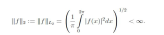
Let L₂ := L2[0, 2π] denote the space of Lebesgue measurable 2π-periodic real functions f with norm

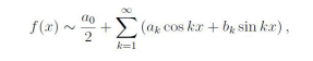
Let 311—1 be the subspace of all trigonometric polynomials of degree n — 1. It is well known that, for any function f E- L₂ with Fourier expansion

the value of its best approximation in L2 by elements of the subspace ℑn−1 is

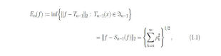
where,

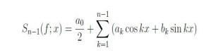
is the partial sum of order n − 1 of the Fourier series for the function f and

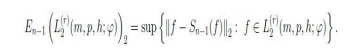
Let denote the norm of the mth.order difference of a function f e L₂: with step h, that is,

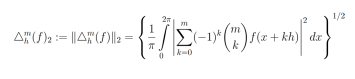
Then

defines the mth-order modulus of continuity of a function f e L₂

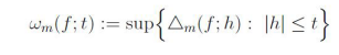
By (r E N; L⁽⁰⁾₂ = L₂) we denote the set of functions f E L₂, whose (r — l)st derivatives are absolutely continuous and f^r E L₂, In Section 3, in defining classes of functions, we characterize the structural properties of a function f E L^r₂ by the rate of convergence to zero of the modulus of continuity of its rth derivative f^(r), defining this rate in terms of the majorant of some averaged quantity ω_m(f^(r); t).

Related Extremal Problems

Extremal problems in the theory of approximation of differentiable periodic functions by trigonometric polynomials in the L₂ space involve the determination of sharp constants in inequalities of Jackson-Stechkin type

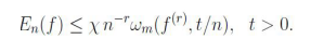
is smaller than the Jackson functional ω_m(f, π/n) and, is apparently more natural for characterizing best approximations E_n−1(f) of periodic functions in L₂.

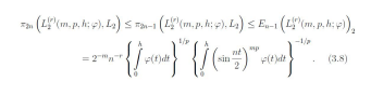
Given these considerations Ligun [2] studied extremal characteristics of the form (in what follows the ratio 0/0 is set equal to zero):

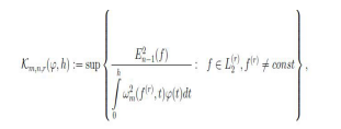
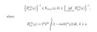
where m, n e N; r Z+; O < h 6 rt/n; 9(t)> 0 is integrable on the segment [0, h]. He showed that

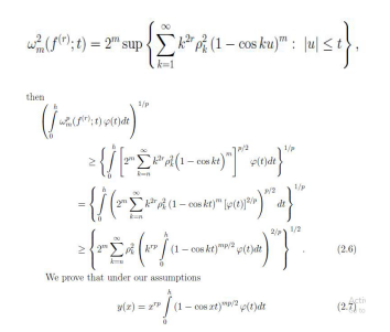
In order to generalize the results of [2], using the scheme of reasoning in Pinkus [3, pp.104-107], Shabozov and Yusupov [4] introduced the extremal characteristic

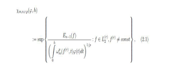
where 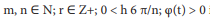is integrable on the segment [O, h], and for O < p 6 2 proved the inequality

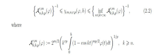
In the calculation of the exact values of the n-widths of classes of functions directly from (2.1), and in connection with the accuracy of (2.2) there is a need to establish the equality

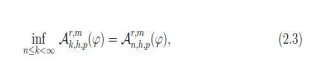
for any positive integrable functions φ on the segment [0, h]. In general, the verification of (2.3) is not always possible. For some specific weight functions φ, condition (2.3) is proved in [5]. Obviously, equation (2.3) depends on the structural properties of the weight function φ. A natural question arises: what structural and differential properties must a function φ have in order to satisfy (2.3)? The answer to the question is contained in the following statement.

Theorem 2.1:Suppose that the weight function φ (t) defined on [0, h] is non-negative and continuously differentiable thereon. If, for and every t E [0, h] we have

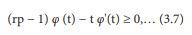
(rp − 1)φ(t) − tφ'(t) ≥ 0, (2.4)

then, for any m, n e N and Wn we have the equality

There is a function const, realizing the upper bound in (2.1) equal to (2.5).

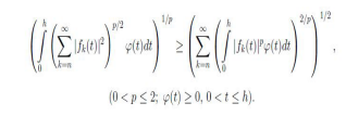
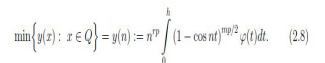
Proof:We use the following simplified version of Minkowski’s inequality [3, p.104]

Indeed, bearing in mind that for any function f E L^(r)₂ we have the relation [10]

is a strictly increasing function in the domain Q = { x : x ≥ 0 } and, hence,

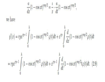
Indeed, differentiating (2.7) and using the elementary identity

Integrating by parts in the last integral of (2.9), the inequality (2.4), we finally obtain

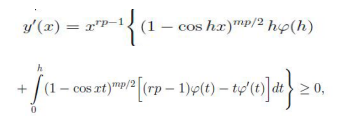
which implies the relation (2.8)

Therefore continuing inequality (2.6), we have

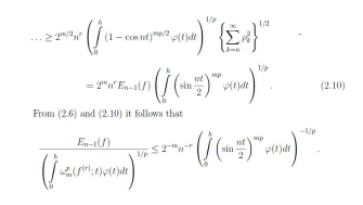
Since the last inequality holds for any f L (r) 2 we have an upper bound for (2.5):

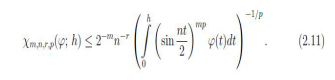
The lower bound in (2.5), valid for all 0 < h ≤ π/n, is obtained by using the function f_o(x) cos nx e L^(r)₂ . We have

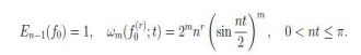
Thus

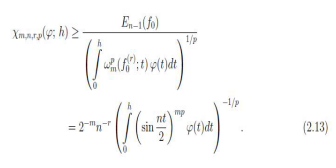
Equation (2.5) is a consequence of (2.11) and (2.12). This completes the proof of Theorem 2.1.

As a particular case of Theorem 2.1 we have:

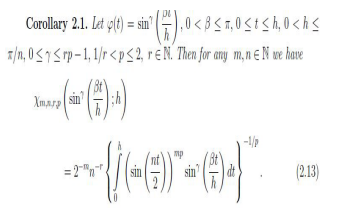
Proof:The parameter values p, r, β, γ, h as in the statement of Corollary 2.1 suffice to verify (2.4). We have

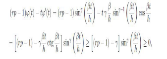
because for the values of the above parameters

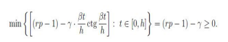
This proves Corollary 2.1.

Corollary 2.1 contains, in particular, the results of [4-8] for different parameters p, γ, β and h.

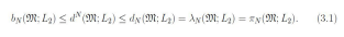
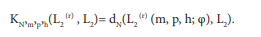
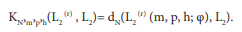
The Statement of the Main Results

We recall the necessary concepts and definitions which will be used later. Suppose that S = {v: ||V|| ≤ 1} is the unit ball in L; is a convex centrally symmetric subset from It; L₂; Λ_NCL₂ is an N.dimensional subspace; Λ^N CL₂ is a subspace of codimension N; L : L₂ + Λ_N is a continuous linear operator taking elements of the space L₂ to Λ_N; and L : L₂ + Λ_N is a continuous linear projection operator from L₂: onto Λ_N, The quantities

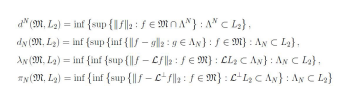
are called, respectively, the Bernstein, Gelfand, Kolmogorov, linear, and projection N-widths in the space L₂ . Since L₂ is a Hilbert space, the N-widths listed above are related by (see, e.g., [3]):

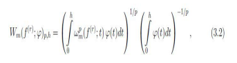
We shall denote by W_m(f^(r); φ)p,h, m E N u {0},0 < p ≤ 2, O ≤ π the pth mean value of the modulus of continuity of mth order of functions f^(r) with weight φ(t) :

and, by L^(r)₂ (m, p, h; φ) we designate the set of functions f E L^(r)₂ for which W_m(f^(r); φ)p,h ≤ ω(f^(r); h),

where C(m, r, p, h) is a positive constant that depends on the values of the parameters in parentheses. With this notation, the search for the smallest constant in the Jackson-Stechkin inequality is equivalent to the problem of computing the exact upper bound

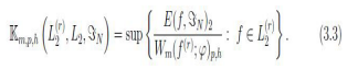
Here we will look for the lowest constant relative to the entire

set of the spaces ℑN CL₂ of fixed dimension N. This will show that the result can not be improved upon by switching to another subspace of the same dimension

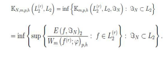
We also put

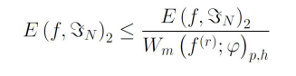
Proposition 3.1:Suppose that h, p > 0, r ℤ₊,.. m, n ∈ N. Then the following inequality holds

Proof. If f ∈ L^(r)₂, φ(t)≥0 is integrable on the segment [O. h] and, W_m(f^(r), φ)p,h = α > 0 then for f1(x) = α⁻¹ f(x), we have Wm(f(r)₁ , φ)p,h = 1. Given the positive homogeneous functional E(f, ℑ N )2 and W_m(f^(r) , φ)p,h, for any 0 < p ≤ 2 and a fixed h> 0 we have

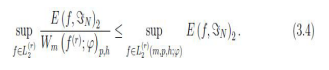
Through (3.4) the lower bound over all subspaces ℑN ⊂ L₂ dimension N we obtain

On the other hand, for any function L^(r)₂ ∈ (m, p, h; φ) bydefinition of the class L^(r)₂ (m, p, h; φ) have an inequality of the form

and as this is true for every subspace ℑN ⊂ L₂ then

Proposition 3.1 follows from (3.5) and (3.6).

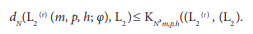
Theorem 3.1. Suppose that the weight function φ (t) defined on the segment [0, h] is non-negative and continuously differentiable thereon. If for some r ∈ ℕ, 1/r < p ≤ 2, and any t ∈ [0, h], we have

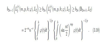
then, for any m, n ∈ ℕ and 0 < h ≤ π/n

where δ_k(·) are any of the k-widths: Bernstein b_k(·), Kolmogorov d_k (·), linear λ_k (·), Gelfand d_k (·) or projection π_k (·). All k–widths are attained by taking the partial sums of the Fourier series S_k−1(f;t).

Proof:From (2.10) and since (3.7) holds, it follows that

Hence, for the width of the projection of class L^(r)₂ (m, p, h; φ), we obtain an upper bound

In order to obtain a lower bound for the Bernstein n-width of L^(r)₂ (m, p, h; φ) we consider the ball

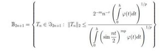
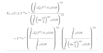
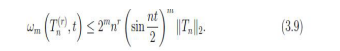
in the (2n+1)–dimensional subspace ℑ2_n+1 of trigonometric polynomials and show that 𝔹_2n+1 ⊂ L^(r)₂ (m, p, h; φ). In [7] it is proved that for an arbitrary polynomial Tn ∈ ℑ_2n+1 for 0 < h ≤ π/n, the inequalit

Elevate both sides of (3.9) to the to the power p, multiply by φ and integrate the result over t in the range from 0 to h. Whence we obtain directly

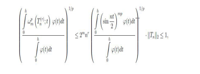
from which 𝔹_2n+1 ⊂ L^(r)₂ (m, p, h; φ). By the definition of the Bernstein n-width we obtain the lower bound

This completes the proof of Theorem 3.1.

As a particular case of Theorem 3.1 we have a result found in [5]. Namely,

Corollary 3.1:Let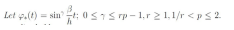

Then the following inequality holds

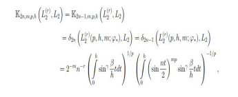
where δ_k(·) are any of the above-listed k-widths

VII.References

---

1. Chernykh NI (1967) On the best L2-approximation of periodic function by trigonometric polynomials. Mat. Zametki 2: 513-22 (in Russian).
2. Ligun AA (1978) Exact inequalities of jackson type for periodic functions in space L2, Mat. Zametki 24: 785-92 (in Russian).
3. Pinkus A (1985) n-Widths in Approximation Theory, SpringerVerlag, Berlin, Heidelberg, New York, Tokyo.
4. Shabozov MSh, Yusupov GA (2011) Best Polynomial Approximations in L2 of Classes of 2π–Periodic Functions and Exact Values of Their Widths, Mat. Zametki 90: 764-75 (in Russian).
5. Shabozov MSh, Yusupov GA (2012) Widths of Certain Classes of Periodic Functions in L2, Journal of Approximation Theory 164: 869-78.
6. Taikov LV (1979) Structural and constructive characteristics of function from L2, Mat. Zametki 25: 217-23 (in Russian).
7. Yusupov GA (2013) Best polynomial approximations and widths of certain classes of functions in the space L2, Eurasian Math. J 4: 120-6.
8. Yusupov GA (2014) Jackson’s – Stechkin’s inequality and the values of widths for some classes of functions from L2, Analysis Mathematica 40: 69-81.