A	B	C	D	E	e	P	p
NA	NB	NC	ND	NE	Ne	NP	Np

Table 1: The population of the nodes of the digraph

	A	B	C	D	E	e	P	p
A	pAA	pAB	pAC	pAD	pAE	0	0	pAp
B	pBA	pBB	pBC	pBD	pBE	pBe	0	pBp
C	pCA	pCB	pCC	pCD	0	0	pCP	pCP
D	pDA	pDB	pDC	pDD	0	pDe	0	pDp
E	pEA	pEB	0	0	pEE	0	0	0
e	0	peB	peC	peD	0	pee	0	0
P	0	0	pPC	0	0	0	pPP	0
p	ppA	ppB	ppC	ppD	0	0	0	ppp

Table 2: Transition matrix

A	B	C	D	E	e	P	p
200	190	240	100	600	130	600	130

Table 3: Following stationary population vector

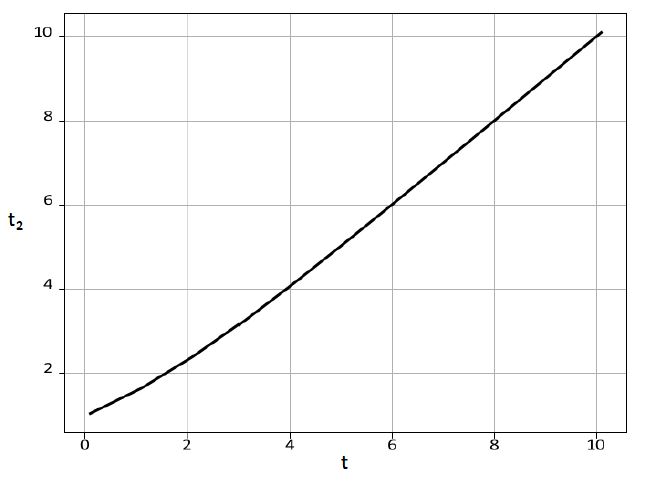Figure 1: Time relationship between two consecutive iterations, see text, equation (14)

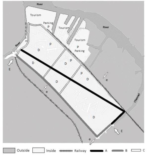Figure 2: Area of interest inside. The outer area has a large number of streets in a grid with different orientations. Since they do not belong to the area where it is desired to control vehicular traffic, they have not been indicated.

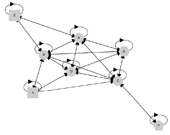Figure 3: A digraph that synthesizes the connections corresponding to those in Figure 2. Note that, assuming the main arteries have dual circulation, the transition from one node to the other can be in either direction

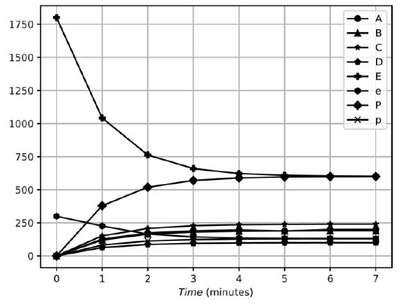Figure 4: Evolution of traffic until steady state is reached

Introduction

The need to predict the behaviour of the trac is necessary and it is a challenging task for the urban planners. Research has been carried out in many articles and reports, among which we cite, for example, the references [1–25] and the books [26,27]. In previous work [28,29], the sites and connecting arteries are represented by digraphs containing vertices and edges; mathematically, they are expressed as stochastic matrices whose diagonal entries represent the number of vehicles at the sites (vertices or nodes) and the off-diagonal entries represent transition probabilities (edges). Now the digraph also has vertices and edges, but the edges represent the transition from one artery to another, and the vertices represent the population of vehicles in each artery. The evolution of an initial configuration is achieved in continuous time using the stochastic matrix developed from the desired steady state. If we multiply an initial vector, whose components represent the one distribution of vehicles, by the stochastic matrix at time t, we obtain the distribution of vehicles at that time. As a first step, we will establish the mathematical properties of the model in the next section.

Mathematical Properties

We will present important new properties of stochastic matrices with application to the construction of Markov chains. In particular, we study the generation of continuous evolutions with respect to a stationary state proposed as optimal, and the uniqueness of the solution will allow its application to numerous specific problems. Let M0 be a stationary stochastic matrix, the continuous evolution generator is defined as

where I is the unitary matrix. Using the generator, we construct a new stochastic matrix,

where t is a parameter defined in non-negative reals that can be associated with time in order to study the evolution of a physical system. A continuous evolution of a system that could be governed by a Markov chain can now be described by M1(t). Obviously the matrices M₀ and M₁(t) commute, since one is a function of the other:

We will prove the following Lemma:

Consider M0 and M1 two stochastic matrices that commute. Let M0 and M1 be two commuting stochastic matrices, let π be the stationary vector of M1, i.e., it is true that π is an eigenvector:

Multiply (4) by M0 on the right,

and with (3)

According to (6) α is an eigenvector of M1, them

After the proof of this property, it is already ensured that the matrix generated in (2) has the desired stationary state, which is determined by M0.

Both matrices have the same stationary vector, i.e. the same stationary state. However, it is possible to iterate the procedures (1) and (2), generating several continuous evolutions. We will now show that they are all equivalent with a suitable time transformation. This is the case when M0 is already a stationary matrix. A second iteration of (2) will be done,

Where M₂(t₂) converges to the same steady state as M₁ and M₀. We now set (2) equal to (9) to obtain a relationship between t and t₂. A condition for (2) to be equal to (9) is as follows,

The fact that e^tG0 = e^t2G2 is verified does not mean that (10) is verified, but the inverse proposition is correct. The series expansion of the e^tG0,

We will calculate the powers of G0, remembering that M0 was considered to be a stationary matrix,

and of course, . The series expansion (11) remains,

Substituting in (10),

Figure 1

This procedure, as shown in Figure 1, can be generalized and in the n−th iteration the time is scaled in the following way,

Then the additional iterations can be converted to the initial iteration by a temporary transformation (15) that does not depend on the matrices.

Figure 2

Example of Transit Application

In the previously cited works [28,29] it was shown, using real values of vehicle mobility in a city, that this mobility can be modelled using a Markov chain. As shown in [29], excellent traffic information is obtained from properly installed surveillance cameras. Now we will see a more ambitious problem than the one solved in the previous works. Instead of a passive observation, now that we are sure that the traffic evolution can be represented by a Markov chain, we will optimise the vehicle movement according to a planned end state. Suppose there is a certain area where many vehicles enter, either for tourism or for a special event. In general, such an area is usually the center of a large city. There will be parking lots in this area, supposedly enough to accommodate the entry of all vehicles, and the problem is to make this entry as orderly as possible to minimize any possible congestion. Instead of concentrating on intersections, as in works [28] and [29], we will now focus on the arteries. The nodes of the digraph are, in this case, the arteries. The purpose of this is to control the number of vehicles on the road. For the sake of fixing ideas, let’s assume a circulation scheme like the one shown in Figure 2. We can assume that the vehicles move in an area of about 2 km x 2 km, although this is not important for the model. Vehicle entry can come from many entrances to the area under consideration, it is a reasonable approximation to assume that the contribution from, say, three key locations. We will also assume that the tourist attraction is located near the main parking lot P, although the vehicles can park at other locations, which we will represent by p. At this point we have come to a key aspect of how to deal with this issue. p will be a node of the digraph, but it will be relatively delocalized in a geographical sense. p is everywhere in the area under consideration where parking is allowed. The same happens with the entrances, we will consider two of them well defined geographically named E, but the third will take into account other multiple accesses that are less relevant and that it will not be necessary to locate exactly, called e.

Inspired by the center of the city of Tigre, we will consider three main access routes to the areas of interest A, B and C, see Figure 1. Circulation through internal roads to the main routes is grouped without differentiation and called D. The model refers only to the inner zone. The outer zone is a reservoir that holds a certain number of vehicles ready to enter the area of interest. Alternative access to this area is difficult because it is surrounded by a river and two railroads. The digraph that corresponds to this is shown in Figure 3.

Figure 3

Table 1

The population of the nodes of the digraph will give information about the number of vehicles circulating in the arteries (A,B,C) or in the inner streets (D), the number of cars stopped in each parking lot (P,p), and the number of incoming and outgoing vehicles (E,e).

Of course, different entrances or different parking lots could be distinguished, and even the number of arteries of interest could be increased, thus increasing the number of elements of the population vector. For the purposes of this example, we will limit ourselves to the suggested nodes. For the purpose of illustration of the behaviour of the model, we shall be content with these eight elements. Initially, there will be a certain number of vehicles at each node. For simplicity, we will assume that there are zero vehicles parked at P and p in the early morning, that there are a certain number of vehicles that normally circulate through the arteries and streets (A, B, C, and D), while the number of vehicles that will enter (E and e) is a certain fraction of those that will enter during the morning. In principle, the next step would be to construct the theoretical transition matrix, see Table 2.

Table 2

Here, however, we will take a different approach. We will use the mathematical tools developed in section (2). To do this, the number of vehicles entering the area should be temporarily controlled to allow them to move from the entrances to the parking lots. This control would initially be performed by traffic agents and, once the model has been optimized, by traffic lights. In this sense, it is necessary to evaluate the distance traveled at a reasonable speed. To fix ideas, dimensions must be established within the area under consideration. The distances of the main arteries are A = 2000m, B = 1900m, C = 2400m, D = 1000m, in the latter case a possible route through the inner streets is considered. The average distance from one of the entrances to the main parking lot P is about 1500m. Assuming a conservative average speed of 30 Km/h, the time required to drive from any driveway to Parking Lot P is approximately 180 seconds. It is reasonable to assume that the cars have an average length of 4m, in addition to 30 km/h, the prescribed distance between vehicles is 2 seconds, or about 16m. We assume that the average vehicle in circulation is approximately 20 meters in length. Considering a circulation capacity of two vehicles in parallel, the circulation capacity in number of vehicles destined for P or p will be at any moment: A = 200v, B = 190v, C = 240v, D = 100v. In the stationary state, it is desirable for the number of entering, circulating, and parked vehicles to be similar. We will propose the following stationary population vector,

Table 3

This would be the stationary case of 2190 vehicles. To get the stationary vector:

Figure 4

For demonstration purposes, we do not take into account the vehicles that naturally circulate in the area of interest. Since the arrival time at the car parks is about 180 seconds, and considering that the parking time can be about 120 seconds, a step to steady state would have been made in 300 seconds. Using we construct the steady state matrix M0 and through (1) and (2) we obtain the continuous evolution matrix that converges to the desired steady state. It shall be verified that for t = 7 the stationary state has been reached by less than one vehicle:

Taking into account the duration of each parking step, steady state would be reached in 21 minutes, see Figure 4. In fact, after 15 minutes, more than 90% of the steady state has been reached.

From now on, vehicle movement will continue as originally requested. Of course, there will be a time limit, which will be set by the car park capacity or the number of vehicles that want to enter.

Conclusions

Although many traffic modeling proposals have been made [1–25], the strong contribution of this work is to propose a desired steady state that avoids possible traffic jams. In the area studied, weekend traffic jams exceed the control capacity of the authorities. Of course, the previous efforts to control the traffic jams must be devoted to a strict control of the flow of vehicles in the entry areas. It is necessary to monitor the traffic and possible accidents by means of cameras and traffic agents equipped with GPS. Here we present a new traffic control method, compatible with this control, based on continuously evolving Markov chains. Mathematically, the algebraic evolution has been established and shown to be a uniquely determined path. Independently of the proposed stationary matrix, the value of time can be modified according to equation (15). There is an implicit difference between a discrete evolution using powers of the transition matrix (Table I) and the continuous evolution proposed in this paper. Note that in the initial transition matrix the possibility of e.g. going from car park P to artery A is zero. However, if the evolution is determined continuously, after one minute the probability of a vehicle going from P to A is pPA = 0.0165...., i.e. it is not zero. In fact, a car can go from P → C → A, and in continuous evolution this possibility is always present due to the multiple paths that eventually connect all the nodes of the digraph, although of course with extremely low probability. As we approach the steady state, this probability is still low but has increased a little: pPA = 0.0912. Under this formalism, the motion of cars behaves like a relatively delocalised cloud. This behaviour can be compared to the concepts of fuzzy sets or quantum probabilities. In addition, these concepts can be extended to the logistics supply chain or to industrial assembly lines. Obviously, the adaptation of a real case would require more precision in the determination of distances and times. The example given in Section 3 is for illustrative purposes only, and it should be noted that in the event of accidents or other events that alter the normal development of vehicular traffic, the proposed steady state must be changed immediately. Controls on access to the area in question shall respond by modifying the means of access.

References

1. Bando M, Hasebe K, Nakayama A, et al. (1994) Structure stability of congestion in traffic dynamics. Japan Journal of Industrial and Applied Mathematics. 11: 203–23.
2. Bando M, Hasebe K, Nakayama A, et al. (1995) Dynamical model of traffic congestion and numerical simulation. Physical review E. 51: 1035.
3. Bando M, Hasebe K, Nakanishi K, et al. (1995) Phenomenological study of dynamical model of traffic flow. Journal de Physique I. 5: 1389–99.
4. Kerner BS, Rehborn H (1997) Experimental properties of phase transitions in traffic flow. Physical Review Letters. 79: 4030.
5. Helbing D, Tilch B (1998) Generalized force model of traffic dynamics. Physical review E. 58: 133.
6. Nagatani T, Nakanishi K, Emmerich H (1998) Phase transition in a difference equation model of traffic flow. Journal of Physics A: Mathematical and General. 31: 5431.
7. De Angelis E (1999) Nonlinear hydrodynamic models of traffic flow modelling and mathematical problems. Mathematical and computer modelling. 29: 83–95.
8. Aw A, Rascle M (2000) Resurrection of” second order” models of traffic flow. SIAM journal on applied mathematics. 60: 916–38.
9. Helbing D (2001) Traffic and related self-driven many-particle systems. Reviews of modern physics. 73: 1067.
10. Nagatani T (2002) The physics of traffic jams. Reports on progress in physics. 65: 1331.10
11. Bellomo N, Delitala M, Coscia V (2002) On the mathematical theory of vehicular traffic flow i: Fluid dynamic and kinetic modelling. Mathematical Models and Methods in Applied Sciences. 12: 1801–43.
12. Greenberg JM (2004) Congestion redux. SIAM Journal on Applied Mathematics. 64: 1175–85.
13. Li ZP, Gong XB, Liu YC (2006) Interdisciplinary physics and related areas of science and technology-an improved car-following model for multiphase vehicular traffic flow and numerical tests. Communications in Theoretical Physics. 46: 367–73.
14. Siebel F, Mauser W (2006) On the fundamental diagram of traffic flow. SIAM Journal on Applied Mathematics. 66: 1150–62.
15. Guang-Han P, Di-Hua S (2009) Multiple car-following model of traffic flow and numerical simulation. Chinese Physics B. 18: 5420.
16. Bressan A, Han K (2011) Optima and equilibria for a model of traffic flow. SIAM Journal on Mathematical Analysis. 43: 2384–417.
17. Bressan A, Liu CJ, Shen W, et al. (2012) Variational analysis of nash equilibria for a model of traffic flow. Quarterly of applied mathematics. 70: 495–515.
18. Goh CY, Dauwels J, Mitrovic N, et al. (2012) Online map-matching based on hidden markov model for real-time traffic sensing applications. In: 2012 15th International IEEE Conference on Intelligent Transportation Systems; IEEE; 776–81.
19. Bressan A, Cani´c S, Garavello M, et al. (2014) Flows on networks: recent results and perspectives.ˇ EMS Surveys in Mathematical Sciences. 1: 47–111.
20. Kiselev A, Kokoreva A, Nikitin V, et al. (2004) Mathematical modelling of traffic flows on controlled roads. Journal of Applied Mathematics and Mechanics. 68: 933–9.
21. Gasser I, Sirito G, Werner B (2004) Bifurcation analysis of a class of ‘car following’traffic models. Physica D: Nonlinear Phenomena. 197: 222–41.
22. Doboszczak S, Forstall V (2013) Mathematical modeling by differential equations. case study: Traffic flow, university of maryland, m3c.
23. Canic S, Piccoli B, Qiu JM, et al. (2015) Runge–kutta discontinuous galerkin method for traffic flow model on networks. Journal of Scientific Computing. 63: 233–55.
24. Bressan A, Han K (2012) Existence of optima and equilibria for traffic flow on networks. arXiv preprint arXiv:12111355.
25. Piccoli B, Tosin A (2009) A review of continuum mathematical models of vehicular traffic. Encyclopedia of Complexity and Systems Science. 9727: 9749.
26. Kerner BS, Lieu H (2005) The physics of traffic: Empirical freeway pattern features, engineering applications; and theory. Physics Today. 58: 54–6.
27. Mahnke R, Kaupuzs J, Lubashevsky I (2009) Physics of stochastic processes: how randomness acts in time. John Wiley & Sons.
28. Otero D, Galetti D, Mizrahi SS (2018) Modeling vehicular traffic networks. part i. Physica A: Statistical Mechanics and its Applications. 509: 97–110.
29. Amadio A, Nicuesa F, Otero D, et al. (2018) Urban vehicular traffic: Fitting the data with a hybrid stochastic model. part ii. Physica A: Statistical Mechanics and its Applications. 509: 469–78.