

Review Article
Volume-1 Issue-1, 2025
A Simple Relationship between the Sample Size and the Number of Independent Variables
-
Received Date: July 02, 2025
-
Accepted Date: July 21, 2025
-
Published Date: July 28, 2025
Journal Information
Abstract
When dealing with multiple regressions for relatively small sample sizes, we often encounter the essential question of how much we should increase the sample size when adding independent variables. Keeping the sample size (n) unchanged and adding an extra independent variable (k), will always result in a better mathematical outcome but will not necessarily yield a better model. This raises the fundamental question of what to do with the sample size for each additional predictor. The majority of the research in this area deals with complex relationships that include the power of the test, the probability of Type II error, the effect size, and other variables. But, when the topic is discussed in introductory statistics courses, certain concepts are not thoroughly explored, and there’s a lack of clear guidance about how to handle the sample size when introducing new independent variables to the regression model. This is especially relevant when moving from the simple linear regression model to the multiple regression one. This paper resolves this by introducing a much-needed simple relationship where the sample size is a function of only the number of independent variables. The model is tested with different values of the significance level to ensure consistency.
Key words
Regression Analysis; Multiple Regression; Number of Predictors
n |
2 |
k |
|||||||||
|
0.05 |
1 |
2 |
3 |
4 |
5 |
6 |
7 |
8 |
9 |
10 |
22 |
|
0.0025 |
-0.0500 |
-0.1083 |
-0.1735 |
-0.2469 |
-0.3300 |
-0.4250 |
-0.5346 |
-0.6625 |
-0.8136 |
42 |
|
0.0263 |
0.0013 |
-0.0250 |
-0.0527 |
-0.0819 |
-0.1129 |
-0.1456 |
-0.1803 |
-0.2172 |
-0.2565 |
62 |
|
0.0342 |
0.0178 |
0.0009 |
-0.0167 |
-0.0348 |
-0.0536 |
-0.0731 |
-0.0934 |
-0.1144 |
-0.1363 |
82 |
|
0.0381 |
0.0259 |
0.0135 |
0.0006 |
-0.0125 |
-0.0260 |
-0.0399 |
-0.0541 |
-0.0687 |
-0.0838 |
102 |
|
0.0405 |
0.0308 |
0.0209 |
0.0108 |
0.0005 |
-0.0100 |
-0.0207 |
-0.0317 |
-0.0429 |
-0.0544 |
122 |
|
0.0421 |
0.0340 |
0.0258 |
0.0175 |
0.0091 |
0.0004 |
-0.0083 |
-0.0173 |
-0.0263 |
-0.0356 |
142 |
|
0.0432 |
0.0363 |
0.0293 |
0.0223 |
0.0151 |
0.0078 |
0.0004 |
-0.0071 |
-0.0148 |
-0.0225 |
162 |
|
0.0441 |
0.0381 |
0.0320 |
0.0258 |
0.0196 |
0.0132 |
0.0068 |
0.0003 |
-0.0062 |
-0.0129 |
182 |
|
0.0447 |
0.0394 |
0.0340 |
0.0285 |
0.0230 |
0.0174 |
0.0118 |
0.0061 |
0.0003 |
-0.0056 |
202 |
|
0.0453 |
0.0405 |
0.0356 |
0.0307 |
0.0258 |
0.0208 |
0.0157 |
0.0106 |
0.0055 |
0.0003 |
2 |
k |
|||||||||
|
1 |
2 |
3 |
4 |
5 |
6 |
7 |
8 |
9 |
10 |
|
n |
|||||||||
0.01 |
102 |
202 |
302 |
402 |
502 |
602 |
702 |
802 |
902 |
1002 |
0.02 |
52 |
102 |
152 |
202 |
252 |
302 |
352 |
402 |
452 |
502 |
0.05 |
22 |
42 |
62 |
82 |
102 |
122 |
142 |
162 |
182 |
202 |
0.10 |
12 |
22 |
32 |
42 |
52 |
62 |
72 |
82 |
92 |
102 |
0.20 |
7 |
12 |
17 |
22 |
27 |
32 |
37 |
42 |
47 |
52 |
0.25 |
6 |
10 |
14 |
18 |
22 |
26 |
30 |
34 |
38 |
42 |
0.50 |
4 |
6 |
8 |
10 |
12 |
14 |
16 |
18 |
20 |
22 |
0.95 |
3 |
4 |
5 |
6 |
7 |
8 |
9 |
10 |
11 |
12 |
0.99 |
3 |
4 |
5 |
6 |
7 |
8 |
9 |
10 |
11 |
12 |
2 |
n |
k |
|
0.01 |
100(k) + 2 |
1 k 10 |
|
0.02 |
50(k) + 2 |
1 k 10 |
|
0.04 |
25(k) + 2 |
1 k 10 |
|
0.05 |
20(k) + 2 |
1 k 10 |
|
0.10 |
10(k) + 2 |
1 k 10 |
|
0.20 |
5(k) + 2 |
1 k 10 |
|
0.25 |
4(k) + 2 |
1 k 10 |
|
0.50 |
2(k) + 2 |
1 k 10 |
|
0.95 |
1(k) + 2 |
1 k 10 |
|
0.99 |
1(k) + 2 |
1 k 10 |
|
2 |
Slope |
0.01 |
100 |
0.02 |
50 |
0.04 |
25 |
0.05 |
20 |
0.10 |
10 |
0.20 |
5 |
0.25 |
4 |
0.50 |
2 |
0.95 |
1 |
0.99 |
1 |
|
Green |
New Model |
k |
n = 8(k) + 50 |
n = 10(k) + 20 |
1 |
58 |
30 |
2 |
66 |
40 |
3 |
74 |
50 |
4 |
82 |
60 |
5 |
90 |
70 |
6 |
98 |
80 |
7 |
106 |
90 |
8 |
114 |
100 |
9 |
122 |
110 |
10 |
130 |
120 |
11 |
138 |
130 |
12 |
146 |
140 |
13 |
154 |
150 |
14 |
162 |
160 |
15 |
170 |
170 |
n |
2 |
k |
|||||||||
|
0.05 |
1 |
2 |
3 |
4 |
5 |
6 |
7 |
8 |
9 |
10 |
3 |
|
-0.9000 |
|
|
|
|
|
|
|
|
|
4 |
|
-0.4250 |
-1.8500 |
|
|
|
|
|
|
|
|
5 |
|
-0.2667 |
-0.9000 |
-2.8000 |
|
|
|
|
|
|
|
6 |
|
-0.1875 |
-0.5833 |
-1.3750 |
-3.7500 |
|
|
|
|
|
|
7 |
|
-0.1400 |
-0.4250 |
-0.9000 |
-1.8500 |
-4.7000 |
|
|
|
|
|
8 |
|
-0.1083 |
-0.3300 |
-0.6625 |
-1.2167 |
-2.3250 |
-5.6500 |
|
|
|
|
9 |
|
-0.0857 |
-0.2667 |
-0.5200 |
-0.9000 |
-1.5333 |
-2.8000 |
-6.6000 |
|
|
|
10 |
|
-0.0687 |
-0.2214 |
-0.4250 |
-0.7100 |
-1.1375 |
-1.8500 |
-3.2750 |
-7.5500 |
|
|
11 |
|
-0.0556 |
-0.1875 |
-0.3571 |
-0.5833 |
-0.9000 |
-1.3750 |
-2.1667 |
-3.7500 |
-8.5000 |
|
12 |
|
-0.0450 |
-0.1611 |
-0.3063 |
-0.4929 |
-0.7417 |
-1.0900 |
-1.6125 |
-2.4833 |
-4.2250 |
-9.4500 |
13 |
|
-0.0364 |
-0.1400 |
-0.2667 |
-0.4250 |
-0.6286 |
-0.9000 |
-1.2800 |
-1.8500 |
-2.8000 |
-4.7000 |
14 |
|
-0.0292 |
-0.1227 |
-0.2350 |
-0.3722 |
-0.5438 |
-0.7643 |
-1.0583 |
-1.4700 |
-2.0875 |
-3.1167 |
15 |
|
-0.0231 |
-0.1083 |
-0.2091 |
-0.3300 |
-0.4778 |
-0.6625 |
-0.9000 |
-1.2167 |
-1.6600 |
-2.3250 |
16 |
|
-0.0179 |
-0.0962 |
-0.1875 |
-0.2955 |
-0.4250 |
-0.5833 |
-0.7813 |
-1.0357 |
-1.3750 |
-1.8500 |
17 |
|
-0.0133 |
-0.0857 |
-0.1692 |
-0.2667 |
-0.3818 |
-0.5200 |
-0.6889 |
-0.9000 |
-1.1714 |
-1.5333 |
18 |
|
-0.0094 |
-0.0767 |
-0.1536 |
-0.2423 |
-0.3458 |
-0.4682 |
-0.6150 |
-0.7944 |
-1.0188 |
-1.3071 |
19 |
|
-0.0059 |
-0.0687 |
-0.1400 |
-0.2214 |
-0.3154 |
-0.4250 |
-0.5545 |
-0.7100 |
-0.9000 |
-1.1375 |
20 |
|
-0.0028 |
-0.0618 |
-0.1281 |
-0.2033 |
-0.2893 |
-0.3885 |
-0.5042 |
-0.6409 |
-0.8050 |
-1.0056 |
21 |
|
-0.0000 |
-0.0556 |
-0.1176 |
-0.1875 |
-0.2667 |
-0.3571 |
-0.4615 |
-0.5833 |
-0.7273 |
-0.9000 |
22 |
|
0.0025 |
-0.0500 |
-0.1083 |
-0.1735 |
-0.2469 |
-0.3300 |
-0.4250 |
-0.5346 |
-0.6625 |
-0.8136 |
23 |
|
0.0048 |
-0.0450 |
-0.1000 |
-0.1611 |
-0.2294 |
-0.3063 |
-0.3933 |
-0.4929 |
-0.6077 |
-0.7417 |
24 |
|
0.0068 |
-0.0405 |
-0.0925 |
-0.1500 |
-0.2139 |
-0.2853 |
-0.3656 |
-0.4567 |
-0.5607 |
-0.6808 |
25 |
|
0.0087 |
-0.0364 |
-0.0857 |
-0.1400 |
-0.2000 |
-0.2667 |
-0.3412 |
-0.4250 |
-0.5200 |
-0.6286 |
26 |
|
0.0104 |
-0.0326 |
-0.0795 |
-0.1310 |
-0.1875 |
-0.2500 |
-0.3194 |
-0.3971 |
-0.4844 |
-0.5833 |
27 |
|
0.0120 |
-0.0292 |
-0.0739 |
-0.1227 |
-0.1762 |
-0.2350 |
-0.3000 |
-0.3722 |
-0.4529 |
-0.5438 |
28 |
|
0.0135 |
-0.0260 |
-0.0687 |
-0.1152 |
-0.1659 |
-0.2214 |
-0.2825 |
-0.3500 |
-0.4250 |
-0.5088 |
29 |
|
0.0148 |
-0.0231 |
-0.0640 |
-0.1083 |
-0.1565 |
-0.2091 |
-0.2667 |
-0.3300 |
-0.4000 |
-0.4778 |
30 |
|
0.0161 |
-0.0204 |
-0.0596 |
-0.1020 |
-0.1479 |
-0.1978 |
-0.2523 |
-0.3119 |
-0.3775 |
-0.4500 |
31 |
|
0.0172 |
-0.0179 |
-0.0556 |
-0.0962 |
-0.1400 |
-0.1875 |
-0.2391 |
-0.2955 |
-0.3571 |
-0.4250 |
32 |
|
0.0183 |
-0.0155 |
-0.0518 |
-0.0907 |
-0.1327 |
-0.1780 |
-0.2271 |
-0.2804 |
-0.3386 |
-0.4024 |
33 |
|
0.0194 |
-0.0133 |
-0.0483 |
-0.0857 |
-0.1259 |
-0.1692 |
-0.2160 |
-0.2667 |
-0.3217 |
-0.3818 |
34 |
|
0.0203 |
-0.0113 |
-0.0450 |
-0.0810 |
-0.1196 |
-0.1611 |
-0.2058 |
-0.2540 |
-0.3063 |
-0.3630 |
35 |
|
0.0212 |
-0.0094 |
-0.0419 |
-0.0767 |
-0.1138 |
-0.1536 |
-0.1963 |
-0.2423 |
-0.2920 |
-0.3458 |
36 |
|
0.0221 |
-0.0076 |
-0.0391 |
-0.0726 |
-0.1083 |
-0.1466 |
-0.1875 |
-0.2315 |
-0.2788 |
-0.3300 |
37 |
|
0.0229 |
-0.0059 |
-0.0364 |
-0.0687 |
-0.1032 |
-0.1400 |
-0.1793 |
-0.2214 |
-0.2667 |
-0.3154 |
38 |
|
0.0236 |
-0.0043 |
-0.0338 |
-0.0652 |
-0.0984 |
-0.1339 |
-0.1717 |
-0.2121 |
-0.2554 |
-0.3019 |
39 |
|
0.0243 |
-0.0028 |
-0.0314 |
-0.0618 |
-0.0939 |
-0.1281 |
-0.1645 |
-0.2033 |
-0.2448 |
-0.2893 |
40 |
|
0.0250 |
-0.0014 |
-0.0292 |
-0.0586 |
-0.0897 |
-0.1227 |
-0.1578 |
-0.1952 |
-0.2350 |
-0.2776 |
41 |
|
0.0256 |
-0.0000 |
-0.0270 |
-0.0556 |
-0.0857 |
-0.1176 |
-0.1515 |
-0.1875 |
-0.2258 |
-0.2667 |
42 |
|
0.0263 |
0.0013 |
-0.0250 |
-0.0527 |
-0.0819 |
-0.1129 |
-0.1456 |
-0.1803 |
-0.2172 |
-0.2565 |
43 |
|
0.0268 |
0.0025 |
-0.0231 |
-0.0500 |
-0.0784 |
-0.1083 |
-0.1400 |
-0.1735 |
-0.2091 |
-0.2469 |
44 |
|
0.0274 |
0.0037 |
-0.0213 |
-0.0474 |
-0.0750 |
-0.1041 |
-0.1347 |
-0.1671 |
-0.2015 |
-0.2379 |
45 |
|
0.0279 |
0.0048 |
-0.0195 |
-0.0450 |
-0.0718 |
-0.1000 |
-0.1297 |
-0.1611 |
-0.1943 |
-0.2294 |
46 |
|
0.0284 |
0.0058 |
-0.0179 |
-0.0427 |
-0.0687 |
-0.0962 |
-0.1250 |
-0.1554 |
-0.1875 |
-0.2214 |
47 |
|
0.0289 |
0.0068 |
-0.0163 |
-0.0405 |
-0.0659 |
-0.0925 |
-0.1205 |
-0.1500 |
-0.1811 |
-0.2139 |
48 |
|
0.0293 |
0.0078 |
-0.0148 |
-0.0384 |
-0.0631 |
-0.0890 |
-0.1163 |
-0.1449 |
-0.1750 |
-0.2068 |
49 |
|
0.0298 |
0.0087 |
-0.0133 |
-0.0364 |
-0.0605 |
-0.0857 |
-0.1122 |
-0.1400 |
-0.1692 |
-0.2000 |
50 |
|
0.0302 |
0.0096 |
-0.0120 |
-0.0344 |
-0.0580 |
-0.0826 |
-0.1083 |
-0.1354 |
-0.1638 |
-0.1936 |
51 |
|
0.0306 |
0.0104 |
-0.0106 |
-0.0326 |
-0.0556 |
-0.0795 |
-0.1047 |
-0.1310 |
-0.1585 |
-0.1875 |
52 |
|
0.0310 |
0.0112 |
-0.0094 |
-0.0309 |
-0.0533 |
-0.0767 |
-0.1011 |
-0.1267 |
-0.1536 |
-0.1817 |
53 |
|
0.0314 |
0.0120 |
-0.0082 |
-0.0292 |
-0.0511 |
-0.0739 |
-0.0978 |
-0.1227 |
-0.1488 |
-0.1762 |
54 |
|
0.0317 |
0.0127 |
-0.0070 |
-0.0276 |
-0.0490 |
-0.0713 |
-0.0946 |
-0.1189 |
-0.1443 |
-0.1709 |
55 |
|
0.0321 |
0.0135 |
-0.0059 |
-0.0260 |
-0.0469 |
-0.0687 |
-0.0915 |
-0.1152 |
-0.1400 |
-0.1659 |
56 |
|
0.0324 |
0.0142 |
-0.0048 |
-0.0245 |
-0.0450 |
-0.0663 |
-0.0885 |
-0.1117 |
-0.1359 |
-0.1611 |
57 |
|
0.0327 |
0.0148 |
-0.0038 |
-0.0231 |
-0.0431 |
-0.0640 |
-0.0857 |
-0.1083 |
-0.1319 |
-0.1565 |
58 |
|
0.0330 |
0.0155 |
-0.0028 |
-0.0217 |
-0.0413 |
-0.0618 |
-0.0830 |
-0.1051 |
-0.1281 |
-0.1521 |
59 |
|
0.0333 |
0.0161 |
-0.0018 |
-0.0204 |
-0.0396 |
-0.0596 |
-0.0804 |
-0.1020 |
-0.1245 |
-0.1479 |
60 |
|
0.0336 |
0.0167 |
-0.0009 |
-0.0191 |
-0.0380 |
-0.0575 |
-0.0779 |
-0.0990 |
-0.1210 |
-0.1439 |
61 |
|
0.0339 |
0.0172 |
-0.0000 |
-0.0179 |
-0.0364 |
-0.0556 |
-0.0755 |
-0.0962 |
-0.1176 |
-0.1400 |
62 |
|
0.0342 |
0.0178 |
0.0009 |
-0.0167 |
-0.0348 |
-0.0536 |
-0.0731 |
-0.0934 |
-0.1144 |
-0.1363 |
63 |
|
0.0344 |
0.0183 |
0.0017 |
-0.0155 |
-0.0333 |
-0.0518 |
-0.0709 |
-0.0907 |
-0.1113 |
-0.1327 |
64 |
|
0.0347 |
0.0189 |
0.0025 |
-0.0144 |
-0.0319 |
-0.0500 |
-0.0687 |
-0.0882 |
-0.1083 |
-0.1292 |
65 |
|
0.0349 |
0.0194 |
0.0033 |
-0.0133 |
-0.0305 |
-0.0483 |
-0.0667 |
-0.0857 |
-0.1055 |
-0.1259 |
66 |
|
0.0352 |
0.0198 |
0.0040 |
-0.0123 |
-0.0292 |
-0.0466 |
-0.0647 |
-0.0833 |
-0.1027 |
-0.1227 |
67 |
|
0.0354 |
0.0203 |
0.0048 |
-0.0113 |
-0.0279 |
-0.0450 |
-0.0627 |
-0.0810 |
-0.1000 |
-0.1196 |
68 |
|
0.0356 |
0.0208 |
0.0055 |
-0.0103 |
-0.0266 |
-0.0434 |
-0.0608 |
-0.0788 |
-0.0974 |
-0.1167 |
69 |
|
0.0358 |
0.0212 |
0.0062 |
-0.0094 |
-0.0254 |
-0.0419 |
-0.0590 |
-0.0767 |
-0.0949 |
-0.1138 |
70 |
|
0.0360 |
0.0216 |
0.0068 |
-0.0085 |
-0.0242 |
-0.0405 |
-0.0573 |
-0.0746 |
-0.0925 |
-0.1110 |
71 |
|
0.0362 |
0.0221 |
0.0075 |
-0.0076 |
-0.0231 |
-0.0391 |
-0.0556 |
-0.0726 |
-0.0902 |
-0.1083 |
72 |
|
0.0364 |
0.0225 |
0.0081 |
-0.0067 |
-0.0220 |
-0.0377 |
-0.0539 |
-0.0706 |
-0.0879 |
-0.1057 |
73 |
|
0.0366 |
0.0229 |
0.0087 |
-0.0059 |
-0.0209 |
-0.0364 |
-0.0523 |
-0.0687 |
-0.0857 |
-0.1032 |
74 |
|
0.0368 |
0.0232 |
0.0093 |
-0.0051 |
-0.0199 |
-0.0351 |
-0.0508 |
-0.0669 |
-0.0836 |
-0.1008 |
75 |
|
0.0370 |
0.0236 |
0.0099 |
-0.0043 |
-0.0188 |
-0.0338 |
-0.0493 |
-0.0652 |
-0.0815 |
-0.0984 |
76 |
|
0.0372 |
0.0240 |
0.0104 |
-0.0035 |
-0.0179 |
-0.0326 |
-0.0478 |
-0.0634 |
-0.0795 |
-0.0962 |
77 |
|
0.0373 |
0.0243 |
0.0110 |
-0.0028 |
-0.0169 |
-0.0314 |
-0.0464 |
-0.0618 |
-0.0776 |
-0.0939 |
78 |
|
0.0375 |
0.0247 |
0.0115 |
-0.0021 |
-0.0160 |
-0.0303 |
-0.0450 |
-0.0601 |
-0.0757 |
-0.0918 |
79 |
|
0.0377 |
0.0250 |
0.0120 |
-0.0014 |
-0.0151 |
-0.0292 |
-0.0437 |
-0.0586 |
-0.0739 |
-0.0897 |
80 |
|
0.0378 |
0.0253 |
0.0125 |
-0.0007 |
-0.0142 |
-0.0281 |
-0.0424 |
-0.0570 |
-0.0721 |
-0.0877 |
81 |
|
0.0380 |
0.0256 |
0.0130 |
-0.0000 |
-0.0133 |
-0.0270 |
-0.0411 |
-0.0556 |
-0.0704 |
-0.0857 |
82 |
|
0.0381 |
0.0259 |
0.0135 |
0.0006 |
-0.0125 |
-0.0260 |
-0.0399 |
-0.0541 |
-0.0687 |
-0.0838 |
83 |
|
0.0383 |
0.0263 |
0.0139 |
0.0013 |
-0.0117 |
-0.0250 |
-0.0387 |
-0.0527 |
-0.0671 |
-0.0819 |
84 |
|
0.0384 |
0.0265 |
0.0144 |
0.0019 |
-0.0109 |
-0.0240 |
-0.0375 |
-0.0513 |
-0.0655 |
-0.0801 |
85 |
|
0.0386 |
0.0268 |
0.0148 |
0.0025 |
-0.0101 |
-0.0231 |
-0.0364 |
-0.0500 |
-0.0640 |
-0.0784 |
86 |
|
0.0387 |
0.0271 |
0.0152 |
0.0031 |
-0.0094 |
-0.0222 |
-0.0353 |
-0.0487 |
-0.0625 |
-0.0767 |
87 |
|
0.0388 |
0.0274 |
0.0157 |
0.0037 |
-0.0086 |
-0.0213 |
-0.0342 |
-0.0474 |
-0.0610 |
-0.0750 |
88 |
|
0.0390 |
0.0276 |
0.0161 |
0.0042 |
-0.0079 |
-0.0204 |
-0.0331 |
-0.0462 |
-0.0596 |
-0.0734 |
89 |
|
0.0391 |
0.0279 |
0.0165 |
0.0048 |
-0.0072 |
-0.0195 |
-0.0321 |
-0.0450 |
-0.0582 |
-0.0718 |
90 |
|
0.0392 |
0.0282 |
0.0169 |
0.0053 |
-0.0065 |
-0.0187 |
-0.0311 |
-0.0438 |
-0.0569 |
-0.0703 |
91 |
|
0.0393 |
0.0284 |
0.0172 |
0.0058 |
-0.0059 |
-0.0179 |
-0.0301 |
-0.0427 |
-0.0556 |
-0.0687 |
92 |
|
0.0394 |
0.0287 |
0.0176 |
0.0063 |
-0.0052 |
-0.0171 |
-0.0292 |
-0.0416 |
-0.0543 |
-0.0673 |
93 |
|
0.0396 |
0.0289 |
0.0180 |
0.0068 |
-0.0046 |
-0.0163 |
-0.0282 |
-0.0405 |
-0.0530 |
-0.0659 |
94 |
|
0.0397 |
0.0291 |
0.0183 |
0.0073 |
-0.0040 |
-0.0155 |
-0.0273 |
-0.0394 |
-0.0518 |
-0.0645 |
95 |
|
0.0398 |
0.0293 |
0.0187 |
0.0078 |
-0.0034 |
-0.0148 |
-0.0264 |
-0.0384 |
-0.0506 |
-0.0631 |
96 |
|
0.0399 |
0.0296 |
0.0190 |
0.0082 |
-0.0028 |
-0.0140 |
-0.0256 |
-0.0374 |
-0.0494 |
-0.0618 |
97 |
|
0.0400 |
0.0298 |
0.0194 |
0.0087 |
-0.0022 |
-0.0133 |
-0.0247 |
-0.0364 |
-0.0483 |
-0.0605 |
98 |
|
0.0401 |
0.0300 |
0.0197 |
0.0091 |
-0.0016 |
-0.0126 |
-0.0239 |
-0.0354 |
-0.0472 |
-0.0592 |
99 |
|
0.0402 |
0.0302 |
0.0200 |
0.0096 |
-0.0011 |
-0.0120 |
-0.0231 |
-0.0344 |
-0.0461 |
-0.0580 |
100 |
|
0.0403 |
0.0304 |
0.0203 |
0.0100 |
-0.0005 |
-0.0113 |
-0.0223 |
-0.0335 |
-0.0450 |
-0.0567 |
101 |
|
0.0404 |
0.0306 |
0.0206 |
0.0104 |
-0.0000 |
-0.0106 |
-0.0215 |
-0.0326 |
-0.0440 |
-0.0556 |
102 |
|
0.0405 |
0.0308 |
0.0209 |
0.0108 |
0.0005 |
-0.0100 |
-0.0207 |
-0.0317 |
-0.0429 |
-0.0544 |
103 |
|
0.0406 |
0.0310 |
0.0212 |
0.0112 |
0.0010 |
-0.0094 |
-0.0200 |
-0.0309 |
-0.0419 |
-0.0533 |
104 |
|
0.0407 |
0.0312 |
0.0215 |
0.0116 |
0.0015 |
-0.0088 |
-0.0193 |
-0.0300 |
-0.0410 |
-0.0522 |
105 |
|
0.0408 |
0.0314 |
0.0218 |
0.0120 |
0.0020 |
-0.0082 |
-0.0186 |
-0.0292 |
-0.0400 |
-0.0511 |
106 |
|
0.0409 |
0.0316 |
0.0221 |
0.0124 |
0.0025 |
-0.0076 |
-0.0179 |
-0.0284 |
-0.0391 |
-0.0500 |
107 |
|
0.0410 |
0.0317 |
0.0223 |
0.0127 |
0.0030 |
-0.0070 |
-0.0172 |
-0.0276 |
-0.0381 |
-0.0490 |
108 |
|
0.0410 |
0.0319 |
0.0226 |
0.0131 |
0.0034 |
-0.0064 |
-0.0165 |
-0.0268 |
-0.0372 |
-0.0479 |
109 |
|
0.0411 |
0.0321 |
0.0229 |
0.0135 |
0.0039 |
-0.0059 |
-0.0158 |
-0.0260 |
-0.0364 |
-0.0469 |
110 |
|
0.0412 |
0.0322 |
0.0231 |
0.0138 |
0.0043 |
-0.0053 |
-0.0152 |
-0.0252 |
-0.0355 |
-0.0460 |
111 |
|
0.0413 |
0.0324 |
0.0234 |
0.0142 |
0.0048 |
-0.0048 |
-0.0146 |
-0.0245 |
-0.0347 |
-0.0450 |
112 |
|
0.0414 |
0.0326 |
0.0236 |
0.0145 |
0.0052 |
-0.0043 |
-0.0139 |
-0.0238 |
-0.0338 |
-0.0441 |
113 |
|
0.0414 |
0.0327 |
0.0239 |
0.0148 |
0.0056 |
-0.0038 |
-0.0133 |
-0.0231 |
-0.0330 |
-0.0431 |
114 |
|
0.0415 |
0.0329 |
0.0241 |
0.0151 |
0.0060 |
-0.0033 |
-0.0127 |
-0.0224 |
-0.0322 |
-0.0422 |
115 |
|
0.0416 |
0.0330 |
0.0243 |
0.0155 |
0.0064 |
-0.0028 |
-0.0121 |
-0.0217 |
-0.0314 |
-0.0413 |
116 |
|
0.0417 |
0.0332 |
0.0246 |
0.0158 |
0.0068 |
-0.0023 |
-0.0116 |
-0.0210 |
-0.0307 |
-0.0405 |
117 |
|
0.0417 |
0.0333 |
0.0248 |
0.0161 |
0.0072 |
-0.0018 |
-0.0110 |
-0.0204 |
-0.0299 |
-0.0396 |
118 |
|
0.0418 |
0.0335 |
0.0250 |
0.0164 |
0.0076 |
-0.0014 |
-0.0105 |
-0.0197 |
-0.0292 |
-0.0388 |
119 |
|
0.0419 |
0.0336 |
0.0252 |
0.0167 |
0.0080 |
-0.0009 |
-0.0099 |
-0.0191 |
-0.0284 |
-0.0380 |
120 |
|
0.0419 |
0.0338 |
0.0254 |
0.0170 |
0.0083 |
-0.0004 |
-0.0094 |
-0.0185 |
-0.0277 |
-0.0372 |
121 |
|
0.0420 |
0.0339 |
0.0256 |
0.0172 |
0.0087 |
-0.0000 |
-0.0088 |
-0.0179 |
-0.0270 |
-0.0364 |
122 |
|
0.0421 |
0.0340 |
0.0258 |
0.0175 |
0.0091 |
0.0004 |
-0.0083 |
-0.0173 |
-0.0263 |
-0.0356 |
123 |
|
0.0421 |
0.0342 |
0.0261 |
0.0178 |
0.0094 |
0.0009 |
-0.0078 |
-0.0167 |
-0.0257 |
-0.0348 |
124 |
|
0.0422 |
0.0343 |
0.0263 |
0.0181 |
0.0097 |
0.0013 |
-0.0073 |
-0.0161 |
-0.0250 |
-0.0341 |
125 |
|
0.0423 |
0.0344 |
0.0264 |
0.0183 |
0.0101 |
0.0017 |
-0.0068 |
-0.0155 |
-0.0243 |
-0.0333 |
126 |
|
0.0423 |
0.0346 |
0.0266 |
0.0186 |
0.0104 |
0.0021 |
-0.0064 |
-0.0150 |
-0.0237 |
-0.0326 |
127 |
|
0.0424 |
0.0347 |
0.0268 |
0.0189 |
0.0107 |
0.0025 |
-0.0059 |
-0.0144 |
-0.0231 |
-0.0319 |
128 |
|
0.0425 |
0.0348 |
0.0270 |
0.0191 |
0.0111 |
0.0029 |
-0.0054 |
-0.0139 |
-0.0225 |
-0.0312 |
129 |
|
0.0425 |
0.0349 |
0.0272 |
0.0194 |
0.0114 |
0.0033 |
-0.0050 |
-0.0133 |
-0.0218 |
-0.0305 |
130 |
|
0.0426 |
0.0350 |
0.0274 |
0.0196 |
0.0117 |
0.0037 |
-0.0045 |
-0.0128 |
-0.0213 |
-0.0298 |
131 |
|
0.0426 |
0.0352 |
0.0276 |
0.0198 |
0.0120 |
0.0040 |
-0.0041 |
-0.0123 |
-0.0207 |
-0.0292 |
132 |
|
0.0427 |
0.0353 |
0.0277 |
0.0201 |
0.0123 |
0.0044 |
-0.0036 |
-0.0118 |
-0.0201 |
-0.0285 |
133 |
|
0.0427 |
0.0354 |
0.0279 |
0.0203 |
0.0126 |
0.0048 |
-0.0032 |
-0.0113 |
-0.0195 |
-0.0279 |
134 |
|
0.0428 |
0.0355 |
0.0281 |
0.0205 |
0.0129 |
0.0051 |
-0.0028 |
-0.0108 |
-0.0190 |
-0.0272 |
135 |
|
0.0429 |
0.0356 |
0.0282 |
0.0208 |
0.0132 |
0.0055 |
-0.0024 |
-0.0103 |
-0.0184 |
-0.0266 |
136 |
|
0.0429 |
0.0357 |
0.0284 |
0.0210 |
0.0135 |
0.0058 |
-0.0020 |
-0.0098 |
-0.0179 |
-0.0260 |
137 |
|
0.0430 |
0.0358 |
0.0286 |
0.0212 |
0.0137 |
0.0062 |
-0.0016 |
-0.0094 |
-0.0173 |
-0.0254 |
138 |
|
0.0430 |
0.0359 |
0.0287 |
0.0214 |
0.0140 |
0.0065 |
-0.0012 |
-0.0089 |
-0.0168 |
-0.0248 |
139 |
|
0.0431 |
0.0360 |
0.0289 |
0.0216 |
0.0143 |
0.0068 |
-0.0008 |
-0.0085 |
-0.0163 |
-0.0242 |
140 |
|
0.0431 |
0.0361 |
0.0290 |
0.0219 |
0.0146 |
0.0071 |
-0.0004 |
-0.0080 |
-0.0158 |
-0.0236 |
141 |
|
0.0432 |
0.0362 |
0.0292 |
0.0221 |
0.0148 |
0.0075 |
-0.0000 |
-0.0076 |
-0.0153 |
-0.0231 |
142 |
|
0.0432 |
0.0363 |
0.0293 |
0.0223 |
0.0151 |
0.0078 |
0.0004 |
-0.0071 |
-0.0148 |
-0.0225 |
143 |
|
0.0433 |
0.0364 |
0.0295 |
0.0225 |
0.0153 |
0.0081 |
0.0007 |
-0.0067 |
-0.0143 |
-0.0220 |
144 |
|
0.0433 |
0.0365 |
0.0296 |
0.0227 |
0.0156 |
0.0084 |
0.0011 |
-0.0063 |
-0.0138 |
-0.0214 |
145 |
|
0.0434 |
0.0366 |
0.0298 |
0.0229 |
0.0158 |
0.0087 |
0.0015 |
-0.0059 |
-0.0133 |
-0.0209 |
146 |
|
0.0434 |
0.0367 |
0.0299 |
0.0230 |
0.0161 |
0.0090 |
0.0018 |
-0.0055 |
-0.0129 |
-0.0204 |
147 |
|
0.0434 |
0.0368 |
0.0301 |
0.0232 |
0.0163 |
0.0093 |
0.0022 |
-0.0051 |
-0.0124 |
-0.0199 |
148 |
|
0.0435 |
0.0369 |
0.0302 |
0.0234 |
0.0165 |
0.0096 |
0.0025 |
-0.0047 |
-0.0120 |
-0.0193 |
149 |
|
0.0435 |
0.0370 |
0.0303 |
0.0236 |
0.0168 |
0.0099 |
0.0028 |
-0.0043 |
-0.0115 |
-0.0188 |
150 |
|
0.0436 |
0.0371 |
0.0305 |
0.0238 |
0.0170 |
0.0101 |
0.0032 |
-0.0039 |
-0.0111 |
-0.0183 |
151 |
|
0.0436 |
0.0372 |
0.0306 |
0.0240 |
0.0172 |
0.0104 |
0.0035 |
-0.0035 |
-0.0106 |
-0.0179 |
152 |
|
0.0437 |
0.0372 |
0.0307 |
0.0241 |
0.0175 |
0.0107 |
0.0038 |
-0.0031 |
-0.0102 |
-0.0174 |
153 |
|
0.0437 |
0.0373 |
0.0309 |
0.0243 |
0.0177 |
0.0110 |
0.0041 |
-0.0028 |
-0.0098 |
-0.0169 |
154 |
|
0.0438 |
0.0374 |
0.0310 |
0.0245 |
0.0179 |
0.0112 |
0.0045 |
-0.0024 |
-0.0094 |
-0.0164 |
155 |
|
0.0438 |
0.0375 |
0.0311 |
0.0247 |
0.0181 |
0.0115 |
0.0048 |
-0.0021 |
-0.0090 |
-0.0160 |
156 |
|
0.0438 |
0.0376 |
0.0313 |
0.0248 |
0.0183 |
0.0117 |
0.0051 |
-0.0017 |
-0.0086 |
-0.0155 |
157 |
|
0.0439 |
0.0377 |
0.0314 |
0.0250 |
0.0185 |
0.0120 |
0.0054 |
-0.0014 |
-0.0082 |
-0.0151 |
158 |
|
0.0439 |
0.0377 |
0.0315 |
0.0252 |
0.0188 |
0.0123 |
0.0057 |
-0.0010 |
-0.0078 |
-0.0146 |
159 |
|
0.0439 |
0.0378 |
0.0316 |
0.0253 |
0.0190 |
0.0125 |
0.0060 |
-0.0007 |
-0.0074 |
-0.0142 |
160 |
|
0.0440 |
0.0379 |
0.0317 |
0.0255 |
0.0192 |
0.0127 |
0.0063 |
-0.0003 |
-0.0070 |
-0.0138 |
161 |
|
0.0440 |
0.0380 |
0.0318 |
0.0256 |
0.0194 |
0.0130 |
0.0065 |
-0.0000 |
-0.0066 |
-0.0133 |
162 |
|
0.0441 |
0.0381 |
0.0320 |
0.0258 |
0.0196 |
0.0132 |
0.0068 |
0.0003 |
-0.0062 |
-0.0129 |
163 |
|
0.0441 |
0.0381 |
0.0321 |
0.0259 |
0.0197 |
0.0135 |
0.0071 |
0.0006 |
-0.0059 |
-0.0125 |
164 |
|
0.0441 |
0.0382 |
0.0322 |
0.0261 |
0.0199 |
0.0137 |
0.0074 |
0.0010 |
-0.0055 |
-0.0121 |
165 |
|
0.0442 |
0.0383 |
0.0323 |
0.0263 |
0.0201 |
0.0139 |
0.0076 |
0.0013 |
-0.0052 |
-0.0117 |
166 |
|
0.0442 |
0.0383 |
0.0324 |
0.0264 |
0.0203 |
0.0142 |
0.0079 |
0.0016 |
-0.0048 |
-0.0113 |
167 |
|
0.0442 |
0.0384 |
0.0325 |
0.0265 |
0.0205 |
0.0144 |
0.0082 |
0.0019 |
-0.0045 |
-0.0109 |
168 |
|
0.0443 |
0.0385 |
0.0326 |
0.0267 |
0.0207 |
0.0146 |
0.0084 |
0.0022 |
-0.0041 |
-0.0105 |
169 |
|
0.0443 |
0.0386 |
0.0327 |
0.0268 |
0.0209 |
0.0148 |
0.0087 |
0.0025 |
-0.0038 |
-0.0101 |
170 |
|
0.0443 |
0.0386 |
0.0328 |
0.0270 |
0.0210 |
0.0150 |
0.0090 |
0.0028 |
-0.0034 |
-0.0097 |
171 |
|
0.0444 |
0.0387 |
0.0329 |
0.0271 |
0.0212 |
0.0152 |
0.0092 |
0.0031 |
-0.0031 |
-0.0094 |
172 |
|
0.0444 |
0.0388 |
0.0330 |
0.0272 |
0.0214 |
0.0155 |
0.0095 |
0.0034 |
-0.0028 |
-0.0090 |
173 |
|
0.0444 |
0.0388 |
0.0331 |
0.0274 |
0.0216 |
0.0157 |
0.0097 |
0.0037 |
-0.0025 |
-0.0086 |
174 |
|
0.0445 |
0.0389 |
0.0332 |
0.0275 |
0.0217 |
0.0159 |
0.0099 |
0.0039 |
-0.0021 |
-0.0083 |
175 |
|
0.0445 |
0.0390 |
0.0333 |
0.0276 |
0.0219 |
0.0161 |
0.0102 |
0.0042 |
-0.0018 |
-0.0079 |
176 |
|
0.0445 |
0.0390 |
0.0334 |
0.0278 |
0.0221 |
0.0163 |
0.0104 |
0.0045 |
-0.0015 |
-0.0076 |
177 |
|
0.0446 |
0.0391 |
0.0335 |
0.0279 |
0.0222 |
0.0165 |
0.0107 |
0.0048 |
-0.0012 |
-0.0072 |
178 |
|
0.0446 |
0.0391 |
0.0336 |
0.0280 |
0.0224 |
0.0167 |
0.0109 |
0.0050 |
-0.0009 |
-0.0069 |
179 |
|
0.0446 |
0.0392 |
0.0337 |
0.0282 |
0.0225 |
0.0169 |
0.0111 |
0.0053 |
-0.0006 |
-0.0065 |
180 |
|
0.0447 |
0.0393 |
0.0338 |
0.0283 |
0.0227 |
0.0171 |
0.0113 |
0.0056 |
-0.0003 |
-0.0062 |
181 |
|
0.0447 |
0.0393 |
0.0339 |
0.0284 |
0.0229 |
0.0172 |
0.0116 |
0.0058 |
-0.0000 |
-0.0059 |
182 |
|
0.0447 |
0.0394 |
0.0340 |
0.0285 |
0.0230 |
0.0174 |
0.0118 |
0.0061 |
0.0003 |
-0.0056 |
183 |
|
0.0448 |
0.0394 |
0.0341 |
0.0287 |
0.0232 |
0.0176 |
0.0120 |
0.0063 |
0.0006 |
-0.0052 |
184 |
|
0.0448 |
0.0395 |
0.0342 |
0.0288 |
0.0233 |
0.0178 |
0.0122 |
0.0066 |
0.0009 |
-0.0049 |
185 |
|
0.0448 |
0.0396 |
0.0343 |
0.0289 |
0.0235 |
0.0180 |
0.0124 |
0.0068 |
0.0011 |
-0.0046 |
186 |
|
0.0448 |
0.0396 |
0.0343 |
0.0290 |
0.0236 |
0.0182 |
0.0126 |
0.0071 |
0.0014 |
-0.0043 |
187 |
|
0.0449 |
0.0397 |
0.0344 |
0.0291 |
0.0238 |
0.0183 |
0.0128 |
0.0073 |
0.0017 |
-0.0040 |
188 |
|
0.0449 |
0.0397 |
0.0345 |
0.0292 |
0.0239 |
0.0185 |
0.0131 |
0.0075 |
0.0020 |
-0.0037 |
189 |
|
0.0449 |
0.0398 |
0.0346 |
0.0293 |
0.0240 |
0.0187 |
0.0133 |
0.0078 |
0.0022 |
-0.0034 |
190 |
|
0.0449 |
0.0398 |
0.0347 |
0.0295 |
0.0242 |
0.0189 |
0.0135 |
0.0080 |
0.0025 |
-0.0031 |
191 |
|
0.0450 |
0.0399 |
0.0348 |
0.0296 |
0.0243 |
0.0190 |
0.0137 |
0.0082 |
0.0028 |
-0.0028 |
192 |
|
0.0450 |
0.0399 |
0.0348 |
0.0297 |
0.0245 |
0.0192 |
0.0139 |
0.0085 |
0.0030 |
-0.0025 |
193 |
|
0.0450 |
0.0400 |
0.0349 |
0.0298 |
0.0246 |
0.0194 |
0.0141 |
0.0087 |
0.0033 |
-0.0022 |
194 |
|
0.0451 |
0.0401 |
0.0350 |
0.0299 |
0.0247 |
0.0195 |
0.0142 |
0.0089 |
0.0035 |
-0.0019 |
195 |
|
0.0451 |
0.0401 |
0.0351 |
0.0300 |
0.0249 |
0.0197 |
0.0144 |
0.0091 |
0.0038 |
-0.0016 |
196 |
|
0.0451 |
0.0402 |
0.0352 |
0.0301 |
0.0250 |
0.0198 |
0.0146 |
0.0094 |
0.0040 |
-0.0014 |
197 |
|
0.0451 |
0.0402 |
0.0352 |
0.0302 |
0.0251 |
0.0200 |
0.0148 |
0.0096 |
0.0043 |
-0.0011 |
198 |
|
0.0452 |
0.0403 |
0.0353 |
0.0303 |
0.0253 |
0.0202 |
0.0150 |
0.0098 |
0.0045 |
-0.0008 |
199 |
|
0.0452 |
0.0403 |
0.0354 |
0.0304 |
0.0254 |
0.0203 |
0.0152 |
0.0100 |
0.0048 |
-0.0005 |
200 |
|
0.0452 |
0.0404 |
0.0355 |
0.0305 |
0.0255 |
0.0205 |
0.0154 |
0.0102 |
0.0050 |
-0.0003 |
201 |
|
0.0452 |
0.0404 |
0.0355 |
0.0306 |
0.0256 |
0.0206 |
0.0155 |
0.0104 |
0.0052 |
-0.0000 |
202 |
|
0.0453 |
0.0405 |
0.0356 |
0.0307 |
0.0258 |
0.0208 |
0.0157 |
0.0106 |
0.0055 |
0.0003 |
2 |
Slope |
0.01 |
100 |
0.02 |
50 |
0.03 |
33.35 |
0.04 |
25 |
0.05 |
20 |
0.06 |
16.67 |
0.07 |
14.27 |
0.08 |
12.52 |
0.09 |
11.10 |
0.10 |
10 |
0.11 |
9 |
0.12 |
8.35 |
0.13 |
7.67 |
0.14 |
7.15 |
0.15 |
6.67 |
0.16 |
6.25 |
0.17 |
5.90 |
0.18 |
5.56 |
0.19 |
5.21 |
0.20 |
5 |
0.21 |
4.76 |
0.22 |
4.52 |
0.23 |
4.35 |
0.24 |
4.15 |
0.25 |
4 |
0.26 |
3.85 |
0.27 |
3.73 |
0.28 |
3.58 |
0.29 |
3.48 |
0.30 |
3.35 |
0.31 |
3.24 |
0.32 |
3.13 |
0.33 |
3 |
0.34 |
3 |
0.35 |
2.87 |
0.36 |
2.8 |
0.37 |
2.73 |
0.38 |
2.65 |
0.39 |
2.56 |
0.40 |
2.52 |
0.41 |
2.44 |
0.42 |
2.38 |
0.43 |
2.33 |
0.44 |
2.25 |
0.45 |
2.24 |
0.46 |
2.15 |
0.47 |
2.13 |
0.48 |
2 |
0.49 |
2 |
0.50 |
2 |
0.51 |
2 |
0.52 |
2 |
0.53 |
1.90 |
0.54 |
1.85 |
0.55 |
1.85 |
0.56 |
1.8 |
0.57 |
1.76 |
0.58 |
1.75 |
0.59 |
1.67 |
0.60 |
1.67 |
0.61 |
1.65 |
0.62 |
1.62 |
0.63 |
1.58 |
0.64 |
1.56 |
0.65 |
1.52 |
0.66 |
1.52 |
0.67 |
1.48 |
0.68 |
1.48 |
0.69 |
1.48 |
0.70 |
1.44 |
0.71 |
1.42 |
0.72 |
1.37 |
0.73 |
1.34 |
0.74 |
1.34 |
0.75 |
1.35 |
0.76 |
1.33 |
0.77 |
1.27 |
0.78 |
1.25 |
0.79 |
1.25 |
0.80 |
1.25 |
0.81 |
1.24 |
0.82 |
1.2 |
0.83 |
1.2 |
0.84 |
1.15 |
0.85 |
1.15 |
0.86 |
1.15 |
0.87 |
1.15 |
0.88 |
1.13 |
0.89 |
1.10 |
 |
| Figure 1: Analysis of leading cybersecurity standards and frameworks components |
 |
| Figure 2:Seven Stages of Research |
 |
| Figure 3: SME Participation from Various Countries |
 |
| Figure 4: SME Participation from Various Countries |
 |
| Figure 5: Security Standards / Frameworks Implemented in SMEs |
Introduction
The purpose of this paper is to offer a simpler and more basic relationship between the number of independent variables (k) and the size of a sample (n) used in building the multiple regression model. This should prove useful in particular to those with limited knowledge of advanced statistical concepts.
In simple regression, the model focuses on only one predictor to explain the behavior and variability of a dependent variable by examining the variability of this one predictor. The most basic and common model is the simple linear regression one. Certain assumptions are made when using a simple linear regression to model the relationship between the dependent variable (response) and the independent variable (predictor).These assumptions are conditions necessary to draw inferences regarding the model, such as the normal distribution of the errors and the independence of the observations.
A common but important misunderstanding among students and less experienced practitioners who want to evolve the simple regression model to a multiple regression one is the practice of adding another variable while maintaining the same sample size; the misconception is to overlook the challenge posed by multiple predictors such as multicollinearity and the insignificance of such new predictors in the model. The result often appears satisfactory to the user, since they see an increase in the mathematical results, such as the coefficient of determination R2 and the p-value of the hypothesis testing to determine the significance of the model. However, this creates pitfalls and misinterpretation of the real outcome of the outputs and may lead to incorrect use of the model that is built.
Thus, the focus of this paper is to address these issues, and to present a new and simple relationship that explains how to manage the size of a sample for every additional predictor.
This relationship will be analyzed, and results obtained will be presented and discussed. Since I start the framework by evolving the simple linear regression model, I limit my independent variables to ten (k 10). In addition, I vary the level of significance (α) to show the consistency of the model.
The analysis is done by observing the behavior of the coefficients of multiple regression, such as the F-statistic and the coefficient of determination R2, to make sure that the relationship developed satisfy the significance condition of the testing of the model.
This paper serves as a guiding tool for students and practitioners who may lack the required analytical background and skills yet who need statistical analysis for decision-making, hence the effort to steer away from the vague and complex mathematical models. I aim to connect these different concepts in a more straightforward and accessible way to help this large audience obtain more reliable results. The new developed model has the linear form: n = b1 (k) + b0
Contemporary advanced statistical software can be used to answer questions similar to the one addressed here using the complex concepts mentioned earlier, such as the power of the test, the acceptable probability of Type II error, the effect size, and other variables. However, since I am focusing on users and practitioners who do not have the necessary analytical or computing skills, I recognized the need to bridge this gap, leading me to the direction I took.
Prior Literature
Regression analysis is one of the most widely used statistical concepts in almost every domain for the purpose of forecasting and prediction, to find which independent variables are better predictors for a selected dependent variable. Given the contemporary capacity to collect more data, add more predictors, and to build and interpret more complex models, multiple regression has become a more widely used application by a majority of practitioners.
The earliest form of regression was the method of least squares presented by Legendre [19], which is an algebraic technique for fitting linear equations to data. Gauss [13] claimed that he was the first one to come up with the least squares work, where he took it beyond Legendre and succeeded in connecting the method with the principles of probability and normal distribution.
Bartko et al. [2] focused on the importance of statistical power accompanied by nomograms for determining sample size and statistical power for the student’s t-tests, whereas Cohen [6,7] and Erdfelder et al. [9] addressed the continued neglect of statistical power analysis in the research by providing a convenient presentation of required sample sizes. Effect-size indexes and conventional values are given for small, medium, and large effects.
I also find an abundance of work, dating back to Fisher [10], and not limited to Bland and Altman [4]; Rovine and Von Eye [24]; and Rodgers and Nicewander [23] who all addressed different aspects of the simple linear regression model. Fisher focused on the frequency distribution of the values of the correlation coefficient in samples from large populations, whereas Rodgers and Nicewander presented thirteen different formulas, each of which represents a different computational and conceptual definition of the correlation coefficient, r.Rovine and Von Eye expanded on this research by presenting a fourteenth way.
Sample sizes have always been a major topic of research when regression is involved. To mention a few, Fritz and MacKinnon [11] presented the necessary sample sizes for six of the most common and most recommended tests of mediation for various combinations of parameters. Hsieh et al. [15] developed sample size formulae for comparing means or proportions in order to calculate the required sample size for a simple logistic regression model. Maas and Hox [20] used a simulation study to determine the influence of different sample sizes at the group level based on the accuracy of the estimates (regression coefficients and variances) and their standard errors. Zaarour and Melachrinoudis [27] developed a relationship between the sample size, the coefficient of determination, and the level of significance, initially in simple linear regression for relatively small sample sizes and later expanded the relationship to include the number of independent variables in multiple regression.
Moving from the basic simple linear regression model to the more complex multiple regression model creates a few important issues. One of these issues is how to deal with the initial sample size. Oliker [22] stated that the problem of determining the number of independent variables is considered under the assumption that the dependent and independent variables have a joint normal distribution, whereas Knofczynski and Mundfrom [18], and Beaujean [3] used a Monte Carlo simulation to model different scenarios to examine the smallest sample sizes for multiple scenarios for each number of independent variables.
This research primarily focuses on the sample size when we decide to increase the number of independent variables is increased. Extensive research has been conducted in this area. Gatsonis and Sampson [12] provided a formula to calculate the minimum sample size required to ensure the reliability of a multiple linear regression model, as did Mendoza and Stafford [21]. Shieh [25,26] presented multiple relationships in separate research papers. Kelly [17] and Algina and Keselman [1], on the other hand, focused on the relationship between the sample size and the squared multiple correlation coefficients in multiple linear regression. Gatsonis and Sampson used the exact power of the test, rather than an approximation, as well as allowing for the calculation of the minimum sample size for a variety of effect sizes rather than just a single effect size. Mendoza and Stafford also enabled the calculation of the minimum sample size by allowing a variety of effect sizes, but they also considered the distinction between the fixed and the random regression models. Shieh incorporated the correlation between the independent variables, since multicollinearity renders the model less efficient, and additionally took into consideration the possibility of the data being clustered, in cases of observational studies. Kelly stated that the minimum sample size required for a multiple regression model to be reliable depends on the squared multiple correlations in addition to the power of the test and the expected variance of the dependent variable. Furthermore, Bujang et al. [5] developed a relationship for the minimum sample size necessary for the multiple regression model in both experimental and non-experimental studies, using the Power and Sample Size Software.
As mentioned earlier, regression analysis is one of the most applied statistical methods in all scientific fields. Thus, we find research that covers the various aspects in all sectors, including engineering and the medical field. Addressing the determination of the sample size in linear regression analysis, Jan and Shieh [16] improved on the approximate formula of Colosimo et al. [8] by developing a more exact approach that outperformed the approximate methods and offered a useful tool in planning validation studies. The stochastic nature of predictors is taken into account by assuming that they have an identical and normal distribution, whereas the Colosimo et al. approach was adopted a direct replacement of mean values for the predictors.
However, in most of these relationships, the focus is on finding the appropriate sample size by using the desired power of the test, the effect size, and the acceptable probability of a Type II error, in addition to other complex variables which are usually challenging for users who do not have the required advanced mathematical proficiencies.
In this paper, I simplify the relationship between the sample size (n) and the number of independent variables (k) by using just the k to calculate the n. I develop a simple linear relationship between n and k and address the challenge when limited resources are available in collecting a sample. I also tested the model using different levels of significance (α) to ensure reliability and consistency of the results.
Model Development and Solution Procedure
In this section, I introduce the necessary variables used in simple linear regression, then I discuss what it entails to transition to a multiple regression model and highlight the main pitfalls arising from this. Lastly, I introduce a simple relationship to calculate the required sample size, given the number of independent variables, and discuss the results and outputs.
Introduction to Simple Linear Regression Factors and Specifics
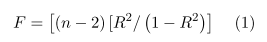
Starting with the coefficient of determination, R2, which is the ratio of the explained variation to the total variation. R2 is used to explain the variability of the dependent variable by considering the variability of the independent variable. It is the used to analyze the fit of the data, using an in-sample performance measure. In addition, to deal with statistical significance, hypothesis testing will have to be performed. One way to obtain this would be to use a statistics similar to the test statistic F. For the simple linear regression case, k = 1 and n ≥3. Hence the relationship between the test statistic F and the R2 is:
Equally, given the significant Fα for a specific (α), I can calculate the values of the critical coefficient of determination R2 to be compared to the R2 values. Starting with the simple linear regression case, I will consider the following:
● According to the central limit theorem, the random sample is considered significant (n ≥ 30), in order for the sample statistics to behave normally.
I will be dealing with relatively small sample sizes since I do not address the work of big data and allowing for our targeted audience’s analytical and computing skills level.
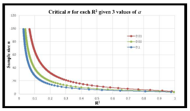
It is worth noting here that I am not referring to the adjusted coefficient of determination Ra2 (which will be discussed later) used with multiple regression, but instead I examine the critical R2 values that would render the model significant. As a result, one can always determine the smallest sample size needed to obtain a significant model given a certain level of significance α, where R2 needs to be equal or higher to a critical value R2. Figure 1 shows these values of n for three specific α values. Consequently, for any value of R2 that we obtain from running our simple linear regression model, we can compare the sample size used to a critical sample size nα. If nis at least equal to the critical value nα, the model will be considered significant.
Transitioning into the Multiple Regression Model
In this section, I address the issues and pitfalls that arise from adding additional predictors to the simple regression model. Once I address those, I introduce in the next section the relationship developed in this paper that will give us a direct and simple insight into how big the sample size needs to be to deal with the additional independent variables.
The complexity of analyzing all the issues in multiple regression is beyond the scope of this paper and its targeted audience. Following is a list of some of those issues:
● For relatively small samples, it is not advisable to keep adding predictors, without changing the size of the sample, as the gap between the coefficient of determination R2 and the adjusted one Ra2 will become more and more significant.
● The mathematical improvement of the outputs is deceiving since it does not necessarily reflect improvement of the model.
● The strong correlation amongst the independent variables, multicollinearity, renders the model less reliable.
● Understanding the desired difference between the true and estimated values of the model.
● Understanding the desired power of the test, and the acceptable probability of the type II error.
● How much to increase the sample size by with every additional k.
When dealing with multiple predictors, I have to ensure that they are not strongly correlated, to avoid redundancy. In addition, merely because the overall model passes the significance test, does not mean that all the predictors are significant and necessary.
Evolving from the simple regression to the multiple regression mode should only be undertaken if it is done correctly. Because our focus in this research is on how to deal with the sample size while making sure the model is significant and avoiding the multicollinearity and the insignificant predictors, the following assumptions are made before moving into the next section:
● No collinearity concerns.
● All added predictors are significant.
● The gap between the coefficient of determination and the adjusted one is accounted for.
Equation (1) can is extended as follows for multiple regression:
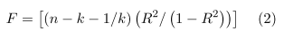
Our purpose in this research is to try to find a new simpler equation that can give us the smallest sample size given the number of independent variables considered in the model, regardless of what level of significance I am dealing with.
Relationship between n and k
As mentioned in the Prior Literature section, there has been a solid amount of work done in finding a relationship between the size of a sample and the number of independent variables considered. Most of these relationships are measured based on their effect size. An effect size is typically a value based on a sample estimate of its corresponding population parameter. In addition, the acceptable probability of the Type I (α) and Type II (β) errors are also considered. As the power of the test (1- β) increases with different levels of α, the sample size will also increase.
I offer a new and simple relationship of n and k, and discuss its impact on the effect size, such as R2, or on the test Statistic F. I start the analysis by looking at the formula for the adjusted coefficient of determination:
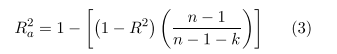
which can be reworked to the following:
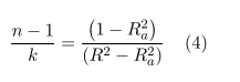
R2 assumes all the independent variables affect the result of the model, whereas Ra2 considers only those variables that actually have an influence on the performance of the model. This is a preliminary endeavor to adjust for the fact that when we add another predictor to a multiple regression, the value of R2 will get larger mathematically, regardless of whether the model becomes more significant. Even though we use the adjusted Ra2 as an out-of-sample performance measure, a smaller gap between the two coefficients is more desirable. Thus, looking back at Equation (4) in order to minimize the gap between the two coefficients:
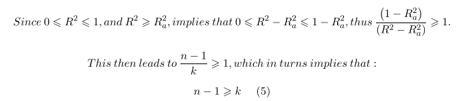
The notion that the degree of freedom (n – 1) is larger than the number of independent variables is not significant on its own. However, the question that really needs to be solved in this research is: how big n needs to be given a k. I start by simulating data for equation (3) to observe for what sample sizes and number of independent variables, does the adjusted coefficient of determination (Ra2) takes on non-negative values given different values of R2.
I chose the following ranges for the simulation:
● n ≥ 3
● 1 ≤ k ≤ 10
● 0.01 ≤ R2 ≤ 0.99, with an increment of 0.01.
Using Excel, I developed 99 different sheets to take into consideration the 99 different values of R2. In each sheet (value of R2), I considered the 10 different values of k and the different values of n. As a result, I obtained a total of more than 200,000 values of Ra2. After applying the condition: n -1 ≥ k, in equation (5) and eliminating all the negative values of Ra2 , I analyzed the remaining values in the following manner: For each value of R2 and k, I found the smallest value of n where the Ra2 starts being non-negative.
Table (1) shows an excerpt of an example of the process with one specific value of R2 = 0.05. The complete table is provided in (Appendix A). Looking at the first row, we notice that for k = 1, n needs to be at least 22 for Ra2 to take on a non-negative value. Not only we are able to find all the n values for a given k, but we also notice a specific trend in the values obtained. We will go over the patterns obtained for all the 99 iterations calculated in the next section.
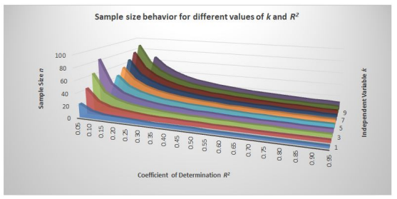
I simulated the same work for the 99 different values of R2. Table (2) and Figure (2) show a summary of the results of the simulation. Results from Table (1) are highlighted in Table(2).
I can see clear patterns of how the sample size behaves when I increase k for the different values of R2. For example, when looking at R2 = 0.01, the pattern is: n = 100(k) + 2. When R2 =0.05, n takes on the following form: n = 20(k) + 2, Or when R2= 0.10, the equation becomes: n = 10(k) + 2. Table (3) shows a summary of some of these patterns:
I can see a pattern with every iteration of the R2, thus the need to develop a general form for these patterns and create an equation that can be used to calculate the sample size as a function of k, regardless of the values of R2.
General Form
These patterns found in the 99 different iterations all have the form n = b1 (k) + b0, where the slope b1 gets smaller as the R2 gets larger. Table (4) shows an excerpt of the 99 different slopes obtained. A detailed table is provided in (Appendix B) showing the 99 different slope obtained for all the values of R2.
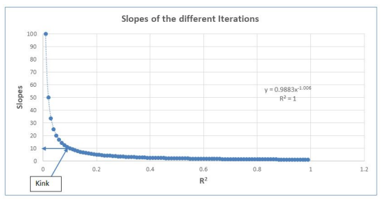
Looking at the distribution of the slopes, the histogram is highly skewed to the right, with the value 10 being the cutoff point where the classes start to dip to the right. In addition, Figure (3) shows the scatter plot obtained graphing all the slopes obtained from the different values of R2.
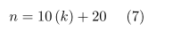
The slope: b1 = 10 is where the kink is observed. This breakthrough allowed for the formulation of the desired model. To complete this model, I needed to calculate the y-intercept. Taking into account the assumptions of normality and having the desired sample size of n ≥ 30 when starting with only one predictor, the y-intercept value was determined to be 20, hence giving us the following new and simplified relationship between n and k:
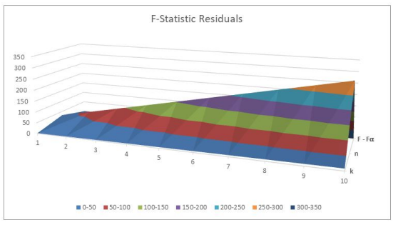
I ran a sensitivity analysis to observe the results of the model. I did this for four different levels of significance to make sure that the model cannot be impacted by changing the alpha. The same behavior emerges regardless of what level of significance used. Figure (4) shows an example of this behavior when ∝ = 0.05. I compared the behavior of the critical value of the F-statistic to the different values of F based on the alpha given. The new simplified relationship between n and k passes the significance test and provides a linear form to calculate the sample size needed given the number of predictors used.
It is vital to mention that the general form of n = 10(k) + 20 not only provides the simplicity and the significance needed to deal with the challenge of increasing the sample size when adding predictors for the multiple regression model but can also handle any number of k, not just up to ten predictors.
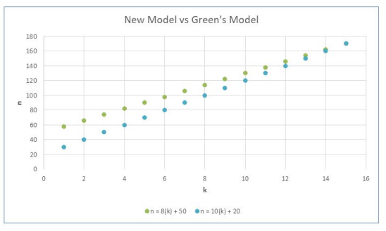
I ran additional Sensitivity Analysis to compare our results to previous models, such as the one from Green [14], who developed a conservative linear form equation: n ≥ 8(k) + 50 and the one from Zaarour et al. [27] who developed a lower bound equation of the coefficient of determination as a function of n and k: R2 > k / (n-1) for multiple regression. I tested my model, and I was able to confirm that my results showed improvement to Green’s well-known rule of thumb as well as satisfied the lower bound condition of R2 of Zaarour’s function.
Table (5) and Figure (5) show the results when comparing the new developed model to Green’s conservative model. I am able to obtain significant results by using a less conservative equation. One of the benefits is that we do not need as big sample sizes (up to k = 15) to obtain the desired results. This is important, especially if we have limited resources to collecting data. It is worth mentioning again that this work deals with relatively small samples due to limitations of resources.
Concluding Remarks
The pivotal question when dealing with multiple regression is how much the sample size must be increased by when adding independent variables. This paper offers a crucial answer in a model that illustrates that sample size is a function of only the number of independent variables, which answers the challenge of what to do with the sample size and how much to increase it by for each additional predictor. The model is developed and tested with different values of the significance level (∝) to make sure we have consistency in the results.
The purpose of the work is to offer a simpler and more basic relationship between the number of independent variables (k) and the size of a sample (n) used in building the multiple regression model. The framework builds the simple linear regression model up, so independent variables are limited to ten (k 10), and the level of significance (∝), is varied to show the consistency of the model.
This paper serves as a guiding tool for students and practitioners who may not have the necessary analytical background and expand from linear regression models to multiple regression models without the aid of highly advanced software that requires specific skills, yet they use statistical analysis for decision-making. This also explains my effort to steer away from vague and complex mathematical models. The model has a linear form n = b1(k) + b0
References
- Algina J, Olejnik S (2000) Determining sample size for accurate estimation of the squared multiple correlation coefficient. Multivariate Behavioral Research 35: 119-36.
- Bartko JJ, Pulver AE, Carpenter WT (1988) The Power of Analysis: Statistical Perspectives. Part II. Psychiatry Research 23: 301-9.
- Beaujean AA (2014) Sample Size Determination for Regression Models Using Monte Carlo Methods in R. Practical Assessment, Research & Evaluation 19: 1-16.
- Bland JM, Altman DG (1996) Measurement Error and Correlation Coefficients. BMJ 313-412.
- Bujang MA, Sa’at N, Sidik TMITAB (2017) Determination of Minimum Sample Size Requirement for Multiple Linear Regression and Analysis of Covariance Based on Experimental and Non-experimental Studies. Epidemiology Biostatistics and Public Health 14: 1-9.
- Cohen J (1992) A Power Primer. Psychological Bulletin 1: 155-9.
- Cohen J (1988) Statistical Power Analysis for the Behavioral Sciences. Hillsdale: Erlbaum.
- Colosimo EA, Cruz FR, Miranda JLO, Woensel TV (2007) Sample Size Calculation for Method Validation using Linear Regression. Journal of Statistical Computation and Simulation, 77: 505-16.
- Erdfelder E, Faul F, Buchner A (1996) GPOWER: A General Power Analysis Program. Behavior Research Methods, Instruments, and Computers 28: 1-11.
- Fisher RA (1915) Frequency Distribution of the Values of the Correlation Coefficient in Samples from an Indefinitely Large Population. Biometrika 4: 507-21.
- Fritz MS, MacKinnon DP (2007) Required Sample Size to Detect the Mediated Effect. Psychological Science 3: 233-9.
- Gatsonis C, Sampson AR (1989) Multiple correlation: Exact power and sample size calculations. Psychological Bulletin 106: 516-24.
- Gauss CF (1809) Theoria motus corporum coelestium in sectionibus conicis solem Ambientum.
- Green SB (1991) How Many Subjects does it Take to do a Regression Analysis? Multivariate Behavioral Research 26: 499‐510.
- Hsieh FY, Bloch DA, Larsen MD (1998) A Simple Method of Sample Size Calculation for Linear and Logistic Regression. Statistics in Medicine 17: 1623-34.
- Jan SL, Shieh G (2019) Sample Size Calculations for Model Validation in Linear Regression Analysis. BioMed Central: Medical Research Methodology 19.
- Kelly K (2008) Sample Size Planning for the Squared Multiple Correlation Coefficient: Accuracy in Parameter Estimation via Narrow Confidence Intervals. Multivariate Behavioral Research 43: 524-55.
- Knofczynski GT, Mundfrom D (2007) Sample Sizes when Using Multiple Linear Regression for Prediction. Educational and Psychological Measurement 68: 431.
- Legendre AM (1805) Nouvelles méthodes pour la détermination des orbites des comètes.Paris: F. Didot.
- Maas CJM, Hox JJ (2005) Sufficient Sample Sizes for Multilevel Modeling. Methodology 3: 86-92.
- Mendoza JL, Stafford KL (2001) Confidence intervals, power calculation, and sample size estimation for the squared multiple correlation coefficient under the fixed and random regression models: A computer program and useful standard tables. Educational and Psychological Measurement 61: 650-67.
- Oliker VI (1978) On the Relationship Between the Sample Size and the Number of Variables in a Linear Regression Mode. Communication in Statistics – Theory and Methods 7: 505-16.
- Rodgers JL, Nicewander WA (1988) Thirteen Ways to Look at the Correlation Coefficient. The American Statistician 1: 59-66.
- Rovine MJ, Von Eye A (1997) A 14th Way to Look at a Correlation Coefficient: Correlation as the Proportion of Matches. The American Statistician 1: 42-6.
- Shieh GA (2006) Exact interval estimation, power calculation, and sample size determination in normal correlation analysis. Psychometrika 71: 529-40.
- Shieh GA (2001) Unified Approach to Power Calculation and Sample Size Determination for Random Regression Models. Psychometrika 72: 347-60.
- Zaarour N, Melachrinoudis E (2019) What’s in a Coefficient? The “Not so Simple Interpretation of R2, for Relatively Small Sample Sizes. Journal of Education and Training Studies 7: 27-40.
Artcle Information
Review Article
Received Date: July 02, 2025
Accepted Date: July 21, 2025
Published Date: July 28, 2025
Journal of Business Management and Economics Statistics
Volume 1 | Issue 1
Citation
Nizar Zaarour (2025) A Simple Relationship between the Sample Size and the Number of Independent Variables. J Bus Manage Econ Stat 1: 104
Copyright
©2025 Nizar Zaarour. This is an open-access article distributed under the terms of the Creative Commons Attribution License, which permits unrestricted use, distribution, and reproduction in any medium, provided the original author and source are credited.

doi: jbme.2025.1.104