

Review Article
Volume-1 Issue-2, 2025
Measuring Persistence of the World Population: A Fractional Integration Approach
-
Received Date: August 05, 2025
-
Accepted Date: August 24, 2025
-
Published Date: August 31, 2025
Journal Information
Abstract
This paper uses fractional integration to measure the de gree of persistence in historical annual data on the world population over the period 1800-2016. The analysis is car ried out for the original series, and for its log transforma tion and its growth rate. The results indicate that the se ries are highly persistent; the estimated values of the di encing parameter are above 1, which implies that shocks have permanent e ects. Endogenous break tests detect one main break shortly a er WWII. The evidence based on the corresponding sub-sample estimation indicates a sharp fall in the degree of dependence between the obser vations in the second sub-sample. Although the original data and their log transformation still exhibit explosive behaviour in that sub-sample, the growth rates are mean reverting, and thus shocks will only have transitory ef fects; moreover, there is a negative time trend. This has implications for the design of policies aimed at contain ing population growth
Key words
Population Growth; Long Memory; Fraction al Integration; Time Trends
Series |
No terms |
With a constant |
With a constant and a linear time trend |
Original |
1.44 (1.34, 1.57) |
1.46 (1.36, 1.59) |
1.46 (1.36, 1.59) |
Log-transformed |
0.98 (0.90, 1.10) |
1.78 (1.66, 1.92) |
1.78 (1.66, 1.92) |
Series |
No terms |
With a constant |
With a constant and a linear time trend |
Original |
1.38 (1.18, 1.72) |
1.41 (1.19, 1.75) |
1.41 (1.20, 1.75) |
Log-transformed |
0.95 (0.81, 1.15) |
1.71 (1.30, 2.20) |
1.71 (1.30, 2.20) |
Series |
No terms |
With a constant |
With a constant and a linear time trend |
White noise |
0.78 (0.66, 0.92) |
0.78 (0.66, 0.92) |
0.78 (0.66, 0.92) |
Autocorrelation |
0.65 (0.30, 1.20) |
0.65 (0.30, 1.20) |
0.65 (0.30, 1.20) |
Series |
N. of breaks |
Break dates |
Original |
3 |
1915; 1948; 1981 |
Series |
N. of breaks |
Break dates |
Original |
1 |
1948 |
Log-transformed |
1 |
1946 |
Growth rate |
1 |
1946 |
|
|||
Series |
No terms |
With a constant |
With a constant and a linear time |
1800 - 1948 |
2.06 (1.95, 2.17) |
3.36 (3.21, 3.59) |
3.37 (3.21, 3.59) |
1949 - 2016 |
1.18 (0.98, 1.49) |
1.14 (0.98, 1.38) |
1.13 (1.00, 1.35) |
|
|||
Series |
No terms |
With a constant |
With a constant and a linear time |
1800 - 1948 |
2.57 (1.85, 2.89) |
2.89 (2.62, 3.14) |
2.88 (2.62, 3.14) |
1949 - 2016 |
0.65 (0.26, 1.02) |
1.20 (1.00, 1.45) |
1.16 (0.99, 1.41) |
|
|||
Series |
No terms |
With a constant |
With a constant and a linear time trend |
1800 - 1948 |
3.36 (3.21, 3.59) |
3925.60 (14.43) |
----- |
1949 - 2016 |
1.14 (0.98, 1.38) |
9737.60. (5.89) |
---- |
|
|||
Series |
No terms |
With a constant |
With a constant and a linear time trend |
1800 - 1948 |
2.89 (2.62, 3.14) |
3925.62 (11.74) |
----- |
1949 - 2016 |
1.20 (1.00, 1.45) |
9758.65. (5.38) |
----- |
|
|||
Series |
No terms |
With a constant |
With a constant and a linear time trend |
1800 - 1948 |
0.99 (0.89, 1.14) |
3.52 (3.07, 4.09) |
3.66 (3.15, 4.15) |
1949 - 2016 |
0.98 (0.83, 1.19) |
1.46 (1.24, 1.76) |
|
|
|||
Series |
No terms |
With a constant |
With a constant and a linear time trend |
1800 - 1948 |
0.93 (0.75, 1.21) |
2.16 (1.09, 2.67) |
2.08 (1.07, 2.63) |
1949 - 2016 |
0.91 (0.62, 1.26) |
1.09 (0.32, 1.59) |
1.08 (0.78, 1.63) |
|
|||
Series |
No terms |
With a constant |
With a constant and a linear time trend |
1800 - 1948 |
3.52 (3.07, 4.09) |
8.265 (184.63) |
0.019 (2.27) |
1949 - 2016 |
|
9.456 (209.80) |
0.055 (2.26) |
|
|||
Series |
No terms |
With a constant |
With a constant and a linear time trend |
1800 - 1948 |
2.08 (1.07, 2.63) |
8.266 (138.84) |
0.018 (2.05) |
1949 - 2016 |
1.08 (0.78, 1.63) |
9.998 (197.59) |
0.020 (2.49) |
|
|||
Series |
No terms |
With a constant |
With a constant and a linear time trend |
1800 - 1948 |
2.29 (2.02, 2.81) |
2.66 (2.15, 3.14) |
2.66 (2.15, 3.15) |
1949 - 2016 |
0.48 (0.29, 0.75) |
0.41 (0.25, 0.68) |
|
|
|||
Series |
No terms |
With a constant |
With a constant and a linear time trend |
1800 - 1948 |
1.40 (0.07, 1.82) |
1.05 (0.06, 1.63) |
1.05 (0.05, 1.64) |
1949 - 2016 |
0.18 (-0.11, 0.70) |
0.15 (-0.09, 1.00) |
0.58 (-0.06, 1.02) |
|
|||
Series |
No terms |
With a constant |
With a constant and a linear time trend |
1800 - 1948 |
2.66 (2.15, 3.14) |
0.0187 (5.16) |
----- |
1949 - 2016 |
|
0.1613 (4.36) |
-0.0025 (-2.45) |
|
|||
Series |
No terms |
With a constant |
With a constant and a linear time trend |
1800 - 1948 |
1.05 (0.05, 1.64) |
0.0173 (2.67) |
0.0015 (2.21) |
1949 - 2016 |
0.58 (-0.06, 1.02) |
0.1761 (4.45) |
-0.0027 (-2.16) |
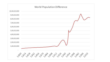 |
| Figure 1: Time series plot |
Introduction
The world population has increased sharply over the history of the planet. 12,000 years ago, it was only 4 million, which would now be the size of a city. Currently, it is 1860 times larg er than at that time (see https://ourworldindata.org/world-population-growth). Its most signi cant growth has occurred in modern times: its size was still under 1 billion at the beginn ing of the 19th century [1]; it then increased sevenfold, the current population representing 6.5% of the total number of individuals born during the entire history of mankind, which was estimated to have been 108 billion [2]. Growth was partic ularly rapid between 1950 and 1987, when the world popula tion increased from 2.5 to 5 billion, the highest growth rate (2.1%) being recorded in 1962; since then, growth has deceler ated, though it remains fast [3]
It should be noted that growth is driven by the di erence be tween births and deaths. Most recently, the increase in deaths has not been matched by a similar one in births, which im plies that the world population growth may halt in the near fu ture. The 'demographic transition' model [4] explains how growth occurs by identifying ve di erent stages, namely: (i) Stage 1: mortality and birth rates are both high; (ii) Stage 2: mortality falls but birth rates are still high; (iii) Stage 3: mortal ity is low and birth rates fall; (iv) Stage 4: mortality and birth rates are both low; (v) Stage 5: mortality is low and there is some evidence of rising fertility (when the fertility rate is low er than two, the population decreases in the long run [3].
The present study provides evidence on the degree of persis tence of the world population. is is measured using a frac tional integration framework, where the fractional di erenc ing parameter is the estimated persistence. is approach is more general than standard ones based on the I(0) stationary versus I(1) no stationary dichotomy since it allows the order of integration to take any real values, including fractional ones. As a result, it encompasses a much wider range of stochastic processes and sheds light on whether or not the se ries is mean-reverting (and thus whether the e ects of shocks are transitory or permanent) and the speed of the dynamic ad justment towards the long-run equilibrium. is method is applied below to analyses the stochastic properties of a world population series starting in 1800, thus obtaining an interest ing set of results with important policy implications.
By analyzing the influential factors that have significantly impacts on the online purchase intention in financial industry, this study enhances the existing literature on the role of purchase perception (i.e. purchase value and risk) in shaping consumer purchase intention in e commerce, as well as intro duces consumer perception as a meditating factor to influence consumers' purchase intention. Amidst the evolving landscape of e-commerce and consumer behaviors, gaps per sist in understanding the determinants of online purchase in tention, particularly within the financial industry. This study aims to address this research gap by comprehensively examin ing the factors infuluencing online purchase intention in the financial sector and exploring the mediating role of consumer perception.
The layout of the following: Section 2 brie y reviews the litera ture on world population trends; Section 3 describes the data and the empirical results: Section 4 o ers some concluding re marks
Literature ReviewThere exist a number of studies aiming to explain the ob served trends in the world population. For instance, [5] anal ysed how small changes in the probabilities of birth, growth, survival, and migration a ect population growth [5]. Speci cally, he showed how, in a system of equations in linear di er ences, the biggest eigenvalue corresponds to the speed of pop ulation growth. A similar approach was used by [6-8] for modelling the world population by age groups. By contrast, [9] considered instead a Markov process with a Leslie matrix for each time interval, and concluded that the world popula tion is log-normal, which is consistent with models of geomet ric growth including non-negative growth. A logistic model was instead estimated by [10] to capture the behaviour of both life expectancy and fertility; however, they could not reach de nite conclusions regarding the future path of the world population
Stochastic demography models have provided new insights in to the likely e ects of increased environmental variability on population trends [11,12] focused instead on the factors that can a ect population trends by causing a decrease in procrea tion in the long run. [13] Investigated the relationship be tween economic development and population growth and showed the importance of migration and urbanisation as drivers of demographic change. [14] examined the same issue applying fractional integration and co integration methods to historical data for Australia, Chile, Denmark, France, the UK, Italy, and the US from 1820 onwards. ey found that the GDP and population series are highly persistent, but the evi dence on the existence of a long-run equilibrium relationship linking these two variables is mixed, co integration only hold ing in the cases of France, Italy and the UK. Finally, [15] pro vided evidence of a linkage between the total fertility rate and GDP by estimating vector error correction models and carry ing out Granger causality tests.
Based on the above literature it is clear that all except [14] use methodologies that use integer degrees of di erentiation and corresponding to 0 in case of stationary series and 1 in case of non-stationary ones. In fact, [14] is the only one that allows fractional degrees of integration, which permits to consider a higher degree of exibility in the dynamic speci cation of the models. e present study applies the same method, i.e., frac tional integration, to historical data on the world population rather than on the population in individual countries as [14] do and thus provides novel evidence.
Data and Empirical AnalysisThe annual world population series used for the analysis spans the period from 1800 to 2016 and has been obtained from the 'OurWorldinData, which is a project of the Global Change Data Lab, a non-pro t organisation based in the UK (Registered Charity Number 1186433), and is available from the following
website: https://ourworldindata.org/world-population-growth#how-has-world-population-growth-changed-over-time
'OurWorldinData' meticulously ensures the integrity of its da tasets. rough stringent validation processes, the organiza tion meticulously cross-references data from various rep utable sources, employing rigorous data cleaning methodolo gies to rectify any inconsistencies. Additionally, 'OurWorldin Data' diligently addresses concerns about data completeness, utilizing sophisticated interpolation techniques when neces sary, and ensuring consistent data quality across di erent time periods by accounting for changes in data collection methodologies. Recognizing the potential for biases, the or ganization implements comprehensive measures to mitigate their impact, including analysing data from diverse regions and demographic groups. e impeccable reputation of 'Our WorldinData' signi cantly enhances the credibility of our analysis, further supported by sensitivity analyses and thor ough discussions on potential limitations, thereby a rming the robustness of our ndings regarding global population dy namics.
Figure 1 displays the evolution over time of the rst di er enced series. It can be seen that it increased gradually from 1800 till the beginning of the 20th century. It then experi enced a sharp decline during both the First and the Second World Wars, a er which it rose sharply, peaking in the 1980s,before subsiding as a result of a fall in fertility.
We analyse the behaviour of the world population by estimat ing a model with deterministic terms as standard in the unit root literature [33], namely:
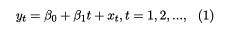
where yt stands for the series of interest, and β0 and β1 are the intercept and the (linear) time trend coe cient;1
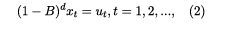
however, unlike in the standard unit root model, in our frac tional integration framework the error term xt is assumed to be integrated of order d, where d can take any real value, including fractional ones, i.e.,
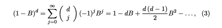
Using a Binomial expansion, one can re-write equation (2), where B is the lag operator, for instance, Bkxt = xt-k, and ut is I(0) [29-32], as follows:
where the higher the value of d is, the higher is the degree of association between observations distant in time. Note that if d = 0 the process exhibits short memory, whilst d>0 implies long memory; if d < 0.5, it is covariance stationary and mean reverting; if 0.5 ≤ d < 1 it is non-stationary but mean rever sion still occurs; if d ≥ 1, the process is explosive.
We then implement the Lagrange Multiplier (LM) test using a version of the Whittle procedure in the frequency domain as in Robinson (1994) for the following null hypothesis:
where do can be any real value. us, under the null (4), the model in (1) and (2) becomes:

and ut is I(0) by assumption. is procedure has important advantages with respect to other methods based on unit roots or fractional integration. The most important one is that the limit distribution is standard normal, unlike what happens with the classical unit root methods [16-18], and this be haviour holds even with the inclusion of the deterministic terms like a constant and a time trend; moreover, do can be any real value, and this allows us consider non stationary cas es, with do ≥ 0.5; nally, this method [19] is the most e cient one in the Pitman sense against local departures. For the func tional form of this procedure, see among others [20-22].
Three model speci cations are considered, namely without deterministic terms, with an intercept only, and with an intercept as well as a linear time trend. Table 1 displays the esti mates of d alongside their 95% condence intervals, for both the original and the log-transformed data, under the assump tion of white noise residuals, whilst Table 2 presents the re sults when allowing for autocorrelation in the error term ut,; in both cases the coe cients in bold are those from the specification selected on the basis of the statistical signi cance of the regressors. Note that for the case of auto correlated residu als we use the exponential spectral model of [23], which is well suited to the framework proposed by [19] and applied in this study. is speci cation approximates AR structures in a non-parametric way, and results in rapidly decaying autocor relation coe cients [24]
The values in bold are those from the model selected on the basis of the statistical signi cance of the regressors.
The values in parenthesis are the condence bands at the 95% level.
The values in bold are those from the model selected on the basis of the statistical signi cance of the regressors.
The values in parenthesis are the condence bands at the 95% level
The values in bold are those from the model selected on the basis of the statistical signi cance of the regressors. The values in parenthesis are the condence bands at the 95% level
Concerning the results with white noise residuals (Table 1), it can be seen that the time trend is not statistically signi cant, and the estimated value of d is greater than 1 for both the orig inal data (1.46) and their log transformation (1.78). As for case of (Bloomeld) autocorrelation in the error term, the results are quite similar, though the estimates of are slightly low er (1.41 for the original data, and 1.71 for the logged ones). We also conducted the analysis for the growth rate, calculated as the rst di erence of the logged values (Table 3).
The parameter d is now estimated to be equal to 0.78 with white noise errors and 0.65 with autocorrelated ones, with the unit root null hypothesis being rejected in the former case in favour of mean reversion (d < 1), but not in the latter one.
Given the long time span, it is possible that breaks have oc curred. erefore we carry out the [25] break tests. sults are reported in Table 4. ese re ree breaks are detected in the case of the original data (1915, 1948 and 1981) and ve in the case of the logged ones (1832, 1880, 1915, 1948 and 1981). e same number of breaks (and break dates) is found in 1946 1946 both cases for the growth rates, which are calculated as the first di erences of the logged series. However, splitting the sample accordingly would yield very short subsamples with unreliable estimates. erefore, we carry out the tests again al lowing for a single break only. is appears to have occurred in 1948 in the case of the original data, and in 1946 for the logged series and the growth rate (Table 5).
The values in bold are those from the model selected on the basis of the statistical signi cance of the regressors.
The values in parenthesis are the condence bands at the 95% level.
The values in bold are those from the model selected on the basis of the statistical signi cance of the regressors.
The values in parenthesis are the condence bands at the 95% level.
The values appearing in bold indicate the signi cant model acccording to the deterministic components. e values in parenthesis are the condence bands at the 95% level.
The values in bold sre those from the model selected on the basis of the statistical signi cance of the regressors.
The values in parenthesis are the confidence bands at the 95% level.
The values in bold are those from the model selected on the basis of the statistical significance of the regressors.
The values in parenthesis are the confidence bands at the 95% level.
The values in bold are those from the model selected on the basis of the statistical significance of the regressors. The values in parenthesis are the confidence bands at the 95% level.
Tables 6, 7 and 8 report the estimated values of d correspond ing to the two subsamples based on the detected breaks for each of the three series (original data, log-transformed ones, growth rates), again for the three speci cations without deter ministic terms, with an intercept only, and an intercept as well as a linear time trend. It is noteworthy that in the case of the original series (Table 6) there is a substantial reduction in the degree of integration a er the break, the estimated value of d decreasing from above 2 (or even 3) before the break to 1 or around 1 a er it. Similar evidence is obtained when using the logged values (Table 7), namely the degree of integration falls sharply a er the break; in addition, there is now a signi cant positive trend in the second subsample. Finally, in the case of the growth rates (Table 8) there is a decrease in the de gree of integration from the rst to the second subsample (from 2.66 to 0.52 with white noise errors and from 1.05 to 0.58 with autocorrelated ones), but the time trend is now neg ative and signi cant in the second subsample regardless of the speci cation for the error term.
Conclusions
This paper uses fractional integration methods to measure the degree of persistence in historical annual data on the world population over the period 1800-2016. The analysis is carried out for the original series, and also for its log transfor mation and its growth rate. The results indicate that the series considered are highly persistent; in particular, the estimated values of the fractional di encing parameter are above 1, which implies that shocks have permanent e ects. As a ro bustness method, we only employed classical unit root tests, and the results, unsurprisingly did not reject the evidence of nonstationarity. Note, however, that these methods (ADF, 1979; PP, 1988; ERS, 1992) simply consider as model speci ca tions those based on d = 0 and d =1, and numerous studies have demonstrated the low power of these approaches under fractional alternatives [26-28].
It should also be noted that these ndings could be biased in the presence of structural breaks which have been over looked. erefore we also carry out endogenous break tests which suggest that the main break in the data occurred short ly a er the Second World War. The evidence based on the corresponding sub-sample estimation indicates a sharp fall in the degree of dependence between the observations in the se cond sub-sample. However, in the case of the original data and their log transformation they are still above 1, which im plies explosive behaviour and permanent e ects of exogenous shocks; in addition, there is a statistically signi cant positive time trend. By contrast, the growth rate of the world popula tion, though not covariance stationary, is mean-reverting, and thus shocks to this series will only have transitory e ects; moreover, there is a negative time trend. is represents im portant information for policy makers concerned with demo graphic trends, since it suggests that there are already some factors at work (such as a fall in fertility) slowing down growth in the world population; this should be taken into ac count when designing policies aimed at containing popula tion growth owing to the limited resources of the planet.
References
- Kremer M (1993) Population growth and technological change: One million BC to 1990. The Quarterly Journal of Economics, 108: 681-716.
- Haub C (1995) How many people have ever lived on earth?. Population Today, 23: 4-5.
- Roser M, Ritchie H, Ortiz-Ospina E, Rodés-Guirao L (2013) World population growth. Our World in Data.
- Kirk D (1996) Demographic transition theory. Population Studies, 50: 361-87.
- Caswell H (1978) A general formula for the sensitivity of population growth rate to changes in life history parameters. Theoretical Population Biology, 14: 215-30
- Emlen JM (1970) Age specificity and ecological theory. Ecology, 51: 588-601.
- Goodman LA (1971) On the sensitivity of the intrinsic growth rate to changes in the age-specific birth and death rates. Theoretical Population Biology, 2: 339-54.
- Hamilton WD (1966) The moulding of senescence by natural selection. Journal of Theoretical Biology, 12: 12-45.
- Tuljapurkar SD, Orzack SH (1980) Population dynamics in variable environments I. Long-run growth rates and extinction. Theoretical Population Biology, 18: 314-42.
- Marchetti C, Meyer PS, Ausubel JH (1996) Human popu lation dynamics revisited with the logistic model: how much can be modeled and predicted?. Technological Forecasting and Social Change, 52: 1-30.
- Boyce MS, Haridas CV, Lee CT (2006) NCEAS Stochastic Demography Working Group. Demography in an increasing ly variable world. Trends in Ecology & Evolution, 21: 141-8.
- Lutz W, Qiang R (2002) Determinants of human population growth. Philosophical Transactions of the Royal Society of London. Series B: Biological Sciences, 357: 1197-210.
- Birdsall N (1988) Economic approaches to population growth. Handbook of Development Economics, 1: 477-542.
- Climent FJ, Meneu R (2004) Demography and economic growth in Spain: a time series analysis. Available at SSRN 482222.
- Dickey DA, Fuller WA (1979) Distributions of the estimators for autoregressive time series with a unit root, Journal of American Statistical Association, 74: 427-81
- Phillips PCB, P Perron (1988) Testing for a unit root in time series regression, Biometrika 75: 335-46.
- Elliot G, TJ Rothenberg, JH Stock (1996) E cient tests for an autoregressive unit root, Econometrica 64: 813-36.
- Robinson PM (1994) E cient tests of nonstationary hy potheses. Journal of the American Statistical Association, 89: 1420-37.
- Gil-Alana LA, Robinson PM (1997) Testing of unit root and other nonstationary hypotheses in macroeconomic time series. Journal of Econometrics, 80: 241-68.
- Gil-Alana LA, Moreno A (2012) Uncovering the US term premium: an alternative route. Journal of Banking & Finance, 36: 1181-93.
- Abbritti M, Gil-Alana LA, Lovcha Y, Moreno A (2016) Term structure persistence. Journal of Financial Economet rics, 14: 331-52.
- Bloomeld P (1973) An exponential model for the spec trum of a scalar time series. Biometrika, 60: 217-26.
- Gil-Alana LA (2004) The use of the Bloomeld model as an approximation to ARMA processes in the context of frac tional integration. Mathematical and Computer Modelling, 39: 429-36
- Bai J, Perron P (2003) Computation and analysis of multi ple structural change models. Journal of Applied Economet rics, 18: 1-22.
- Diebold FX, Rudebush GD (1991) On the power of Dickey‐ Fuller tests against fractional alternatives. Economics Letters, 35: 155-60.
- Hassler U, Wolters J (1994) On the power of unit root tests against fractional alternatives. Economics Letters, 45: 1-5.
- Lee D, Schmidt P (1996) On the power of the KPSS test of stationarity against fractionally-integrated alternatives. Jour nal of Econometrics, 73: 285-302.
- Granger CW (1980) Long memory relationships and the aggregation of dynamic models. Journal of Econometrics, 14: 227-38.
- Granger CWJ (1981) Some properties of Time Series data and their use in Econometric Model Speci cation, Journal of Econometrics, 16: 121-31.
- Granger CW, Joyeux R (1980) An introduction to long memory time series models and fractional di erencing. Jour nal of Time Series Analysis, 1: 15-29.
- Hosking JRM (1985) Fractional di erencing modeling in hydrology 1. JAWRA Journal of the American Water Re sources Association, 21: 677-82.
- Bhargava A (1986) On the theory of testing for unit roots in observed time series. The Review of Economic Studies, 53: 369-84.
- United Nations, Department of Economic and Social Af fairs, Population Division (2017). World Population Prospects: The 2017 Revision, DVD Edition.
Artcle Information
Review Article
Received Date: August 05, 2025
Accepted Date: August 24, 2025
Published Date: August 31, 2025
Journal of Business Management and Economics Statistics
Volume 1 | Issue 2
Citation
Gil-Alana, L. A., Caporale, G. M., Infante, J., & del Rio, M. (2025). Measuring Persistence of the World Population: A Fractional Integration Approach. Journal of Business Management and Economic Statistics, 1: 201
Copyright
©2025 Gil-Alana, L. A., Caporale, G. M., Infante, J., & del Rio. This is an open-access article distributed under the terms of the Creative Commons Attribution License, which permits unrestricted use, distribution, and reproduction in any medium, provided the original author and source are credited.

doi: jbme.2025.1.201